Temporal Bone Imaging Technique
This chapter on the technique for imaging the temporal bone is a practical “how to” written in two parts. In the first part, we explain how to image the temporal bone: how to run the hardware and obtain the images. We present the imaging modalities and technical parameters routinely used for imaging of the temporal bone. In addition, we provide guidelines for the technologist or radiologist as to how to determine which parameters to enter into the computed tomography (CT) or magnetic resonance imaging (MRI) scanner. In the second part, we explain how to read and report the results of temporal bone imaging studies. Here we provide a plan of action for the radiologist who, faced with a request for a temporal bone imaging study on a particular patient, must protocol the case, interpret the images, and report the findings in a way that answers the referring clinician’s questions. The major indications for imaging of the temporal bone are thus reviewed, and protocols, interpretive strategies, and template reports are provided for each of these indications.
Imaging Modalities and Technical Parameters
CT and MRI are primarily used for imaging of the temporal bone. We first present the standard technique and protocols most often used, then review the special considerations for both modalities. A brief overview of the roles of plain radiographs, ultrasound (US), positron emission tomography (PET), and PET/CT is given at the end of this section.
Computed Tomography
Routine Technique
The patient is placed supine in the gantry and positioned to place the lens of the eye as far as possible out of the pathway of the x-ray beam to minimize exposure to the lens. Gantry tilt may need to be avoided to facilitate image reconstruction and reformats. A lateral topogram is then performed. The scan excursion is plotted from the arcuate eminence (the summit of the temporal bone) through the mastoid tip.
The anatomy and pathology of the temporal bone involve small structures; resolution is thus highly important. Collimation is of optimal importance to achieve high resolution.
We routinely use a collimator of 0.6 mm and most commercially available units can be collimated to at least 1 mm. Collimation wider than 1 mm is not usually used, as the resolution is often insufficient.
For 40 to 64 detector scanners, the effective mAs (defined as the mA × the gantry cycle time/helical pitch) is adjusted according to the age and head size. Usually, it is 150 effective mAs (CTDIvol [volume CT dose index] 34 milligray [mGy]) for neonates, 200 effective mAs (CTDIvol 45 mGy) for children ages 1 to 10 years, 250 effective mAs (CTDIvol 57 mGy) for adolescents, and 320 (CTDIvol 72 mGy) for adults. The gantry cycle time is set at 1 cycle or gantry rotation/second. The kilovolt peak (kVp) is usually 120.
A helical mode is chosen. Although traditionally, some imagers maintain that nonhelical scans provide better resolution, it is our experience that the difference in resolution between nonhelical and helical acquisitions at thin collimation is not appreciable, and helical acquisitions allow for clearer coronal or oblique reformats and decrease susceptibility to motion artifact.
Intravenous (IV) contrast is usually of the low osmolar type; it is administered by power injector at standard doses of 1 mL/lb to a maximum of 80 to 100 mL for adults. IV contrast is used for the evaluation of vascular pathology (e.g., dissection, tumors) and may be considered for some types of infections such as coalescent mastoiditis or for the evaluation of abscesses. However, it is not routinely used to evaluate for otomastoiditis or hearing loss.
The raw data from each ear are separated and reconstructed into 0.6 mm (slice thickness) axial images in bone algorithm at a dual field of view (DFOV) of 100 mm that effectively magnifies the images. Then the 0.6 mm images for each ear are brought up on the CT scanner console, where the raw data are displayed in three orthogonal planes. The technologist scrolls through the sagittal data to find an image where the anterior and posterior limbs of the lateral semicircular canal are displayed in cross section (Fig. 1.1). An axial dataset is then made in a plane parallel to the lateral semicircular canal (LSCC). The technologist “connects the two dots” of the LSCC and makes a 0.6 mm (image thickness) × 0.5 (distance between images) axial dataset in this plane parallel to the LSCC; 0.6 × 0.5 mm coronal images are made in a plane perpendicular to the axial images. The raw data are also reconstructed into 2 mm axial images in soft tissue algorithm to include both ears and the brain at 180–210 mm DFOV. This protocol generates seven sets of images, three for each ear—the source 0.6 mm images (in a variable axial plane), the 0.6 mm reformats in the axial plane parallel to the LSCC, the 0.6 mm reformats in the coronal plane, and a set of 2 mm axial images in soft tissue algorithm of the entire scan volume.
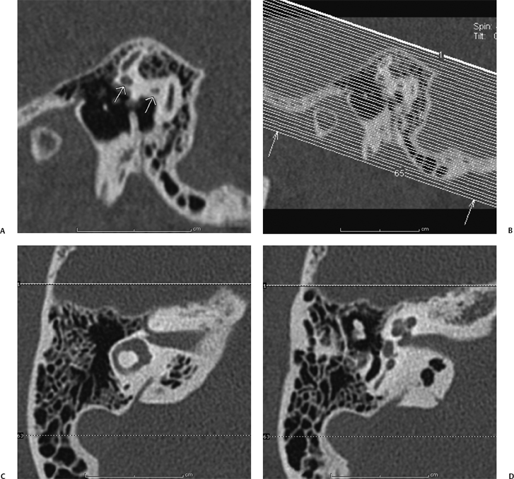
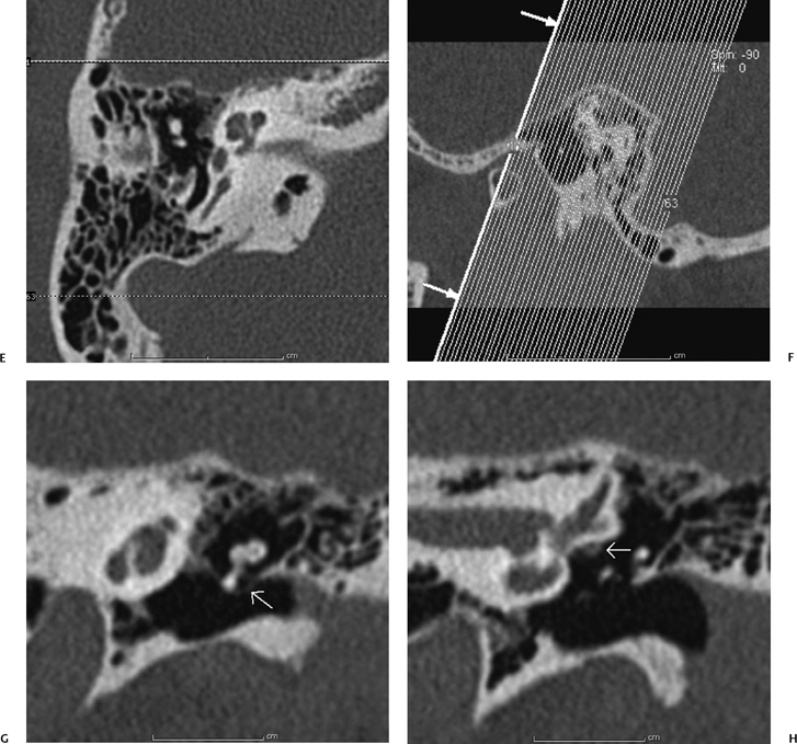
Fig. 1.1 Making the standard axial and coronal computed tomography (CT) dataset. (A) Once the source data are brought up in the three-dimensional (3D) viewer on the scanner console, the sagittal images are scrolled through until a sagittal image through the anterior and posterior limbs (short white arrows) of the lateral semicircular canal (LSCC) are found. (B) A set of axial images is then generated with 0.1 mm overlap parallel to this plane. (C) If the axial reconstructions have been done correctly, the axial dataset should produce an image where the entire lateral semicircular canal is displayed and, as in (D,E), where the cochlear fossette, modiolus, and stapes footplate are clearly delineated. (F) The coronal reconstructions are made in a similar fashion. Starting with the sagittal image in (A), a plane perpendicular to the LSCC is established, and the coronal reformats are made along this plane. (G) This technique should yield a set of coronal images where Prussak’s space (short white arrow) and (H) the facial nerve canal (short white arrow) are clearly delineated.
Multidetector Computed Tomography Reformats
Multidetector CT provides shorter acquisition times, a decrease in tube current load, and improved spatial resolution.1 Short acquisition is useful in temporal bone imaging to reduce motion artifact, particularly in children who require sedation or are imaged postprandially without pharmacologic sedation. Although the radiation dose with multidetector scanners in high-quality mode remains an issue compared with single detector scanners, the improved spatial resolution allows for high-quality reformats that essentially obviate the need for rescanning the patient in a second coronal plane.1
Reformats may, moreover, be obtained in sagittal or oblique planes to improve the detection of pathology in specific clinical settings such as superior semicircular canal dehiscence (SSCD) as discussed below in the section Vertigo and Dizziness.
Stenvers Reformat
Similar to the method explained above, for making the standard axial and coronal images, the 0.6 mm raw data are brought up on the console viewer in three orthogonal planes: axial, coronal, and sagittal. As above, the technologist scrolls through the sagittal plane until a view of the LSCC is obtained represented by the two “dots” of the anterior and posterior limbs (Fig. 1.2). The axial plane is then established by connecting the two dots. The technologist scrolls through the axial dataset until an image of the summit of the SSC is viewed. The Stenvers reformats are then made by tracing a line perpendicular to the long axis of the summit of the SSC at 0.6 0.5 mm intervals. This plane is effectively perpendicular to the roof of the SSC and displays the roof of the SSC in cross section.
Pöschl Reformat
Similar to the method explained above, for making the standard axial and coronal images, the 0.6 mm raw data are brought up on the console viewer in three orthogonal planes: axial, coronal, and sagittal. As above, the technologist scrolls through the sagittal plane until a view of the LSCC is obtained represented by the two “dots” of the anterior and posterior limbs (Fig. 1.3). The axial plane is then established by connecting the two dots. The technologist then scrolls through the axial dataset until an image of the summit of the SSC is viewed. The Pöschl reformats are then made by tracing a line parallel to the long axis of the summit of the SSC at 0.6 0.5 mm intervals. The line must be made as parallel as possible to the axis of the summit of the SSC. A slight obliquity may spuriously obscure a dehiscence by volume averaging with the temporal bone on either side of the summit of the SSC.
Computed Tomography Arteriography and Computed Tomography Venography
CT arteriography (CTA) or CT venography (CTV) of the temporal bone may be used to evaluate for tinnitus. At our institution, the standard CT protocol for temporal bone imaging is employed, but the injection rate is increased to 3 to 4 cc per second for CTA. A power injector is employed if a 22-gauge IV or larger is available.
Radiation Dose Reduction Techniques and Considerations for Pediatric Patients
Compared with most radiography procedures, CT exams deliver higher radiation dosages to patients. The quantity CTDIvol is used to describe the patient dose. CTDIvol represents the average dose in a given scan volume. When a scan is prescribed, the system displays the CTDIvol in mGy on the console. However, the dose displayed is not the true dose for the specific patient under examination. Instead, it is the dose value when the patient is replaced with an acrylic phantom while the same imaging parameters are used. The head phantom is a cylinder with a diameter of 16 cm and a height of 15 cm.
The effective dose E is used to assess the radiation detriment from partial-body as opposed to whole-body irradiation (e.g., irradiation of only the head or only the abdomen). The effective dose is a weighted sum of the doses to all exposed tissues. E = Σ (wt × Ht), where Ht is the equivalent dose to a specific tissue and wt is the weight factor representing the relative radiosensitivity of that tissue. The unit of effective dose is sievert (Sv). The effective dose for a typical CT exam of the temporal bone is ∼ 1 mSv (i.e., 1/1000 Sv). In comparison, the average effective dose from cosmic rays, radioisotopes in the soil, radon, and so on, is ∼ 3 mSv per year in the United States. The effective dose can be estimated from the dose-length product (DLP = CTDIvol × scan length), which is also displayed on the CT scanner console. The effective dose for a head study in mSv is 0.0021 DLP (mGy cm).2
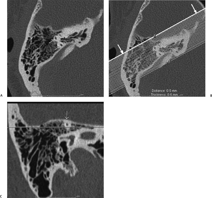
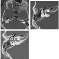
Fig. 1.2 How to make a Stenvers reformat. (A) Once the source data are brought up in the three-dimensional viewer on the scanner console, the axial images are scrolled through until an image through the summit of the superior semicircular canal (SSC; short white arrows) is found. (B) The Stenvers reformats are made in a plane perpendicular to the long axis of the SSC, and (C) should yield a cross-sectional view of the SSC (short white arrow).
Radiation Risks The biological effect of radiation is either deterministic or stochastic. The deterministic effect will not occur unless a threshold dose is exceeded. However, the stochastic effects may occur at any dose level, and the probability of occurrence increases with dose linearly according to the linear nonthreshold dose–response model.3
For CT of the temporal bone, the primary concern for deterministic effect is the dose to the lens. The minimum dose required to produce a progressive cataract is 2 Gy in a single exposure.4 If the lens is in the direct x-ray beam, the dose to the lens from CT of the temporal bone is in the range of 0.03 to 0.06 Gy, but it could be as high as 0.13 Gy. If the patient is positioned in such a way that the lens is outside the direct x-ray beam, the dose is in the order of 0.003 Gy.5 Although the typical dose to the lens from a single CT scan is much lower than the threshold value for a cataract, multiple nonoptimized scans in a short time with the lens in the x-ray beam can result in a lens dose close to the threshold. Every effort should be made to keep the lens outside a direct x-ray beam if it is possible.
Fig. 1.3 How to make a Poschl reformat. (A) Once the source data are brought up in the three-dimensional viewer on the scanner console, the axial images are scrolled through until an image through the summit of the superior semicircular canal (SSC) is found. (B) The Poschl reformats are made in a plane perpendicular to the long axis of the SSC, and (C) should yield a view of the entire excursion of the SSC (short white arrows) from anterior to posterior.
Stochastic effects include carcinogenesis and the induction of genetic mutations. Children are inherently more sensitive to radiation because they have more dividing cells, and radiation acts on dividing cells. Also, children have more time to express a cancer than do adults.6
Factors Influencing the Patient Dose The CT scanning protocols should be optimized such that the quality of images is sufficient for diagnosis and the patient dose is kept as low as reasonably achievable (ALARA). To get the best balance of the image quality and patient dose, it is important to understand the effects of imaging parameters on the dose and imaging quality.
Patient dose depends on three factors: equipment-related factors, patient-related factors, and application-related factors.
The dose is strongly dependent on patient size. If the same technique is used to image the heads of an average adult and a newborn, the dose to the newborn is significantly higher.
Imaging parameters such as kVp, mAs (the product of the tube current and the time in seconds per rotation), and pitch (the table travel per rotation divided by the total x-ray beam width) are selected by the operator.
If all other parameters are fixed, the patient dose is proportional to the effective mAs which is defined as the mAs (mA × seconds per rotation) divided by the pitch.
The dependency of dose to kVp is more complicated. In general, the dose increases as a power function of kVp (D kVpp) if all other parameters are fixed. The value of p is in the order of 2 to 3 depending on the type of scanner.
Image Quality Image quality is characterized by spatial resolution, contrast resolution, image noise, and other quantities. It is difficult to use a single variable to characterize completely the quality of an image. However, in practice, image noise has been widely used to judge the CT image quality because the detectability of low-contrast objects is strongly dependent on the contrast-to-noise ratio. The standard deviation of a region of interest (ROI) in the image is usually used to represent the noise. In CT, for a given reconstruction kernel, the noise is primarily due to the fluctuation of the x-ray photons reaching the detector. The noise is approximately inversely proportional to the square root of the patient dose. To reduce the noise by a factor of 2, the dose must be increased by a factor of 4. In general, image quality is better when the patient dose is increased.
Strategy for Dose Reduction To optimize the CT technique, the image quality required for the specific indication is assessed based on the radiologist’s experience. The imaging parameters are then selected based on the patient size and organ type under exam such that the required image quality is achieved, while the patient dose is kept as low as possible. Weight- or age-based pediatric protocols should be established and special attention should be paid to children under age 2 because their heads are small and under rapid development.
In general, the technologist and radiologist should keep in mind that
Dose mA, time in seconds per rotation of the gantry, kVp2.5, and 1/pitch and adjust these parameters to reduce dose, while maintaining image quality.
Often these adjustments are done empirically, and the technique described above (see Routine Technique section) represents our experience with such adjustments.
Magnetic Resonance Imaging
Routine Technique
The standard MRI protocol for evaluation of the temporal bone in adults is detailed below for a 1.5T (Tesla) magnet.
The patient is placed in the supine position in the head coil.
Sagittal T1-weighted, axial T2-weighted, axial fluid attenuated inversion recovery (FLAIR), and axial diffusion weighted images (DWIs) are obtained through the whole brain.
Axial T1-weighted images are obtained through the temporal bone from the arcuate eminence through the mastoid tip using the following parameters: TR (time to repetition) = 300 milliseconds; TE (echo time) = 12 milliseconds; flip angle = 90 degrees; slice thickness = 3 mm; distance factor = 0.10; matrix = 192 × 256 (phase to frequency encoding steps); FOV = 180 mm; two acquisitions, one saturation, time = 3 minutes, 15 seconds.
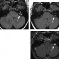
Axial CISS (constructive interference in steady state; Siemens AG, Berlin/Munich, Germany) or 3D (three-dimensional) FIESTA (fast imaging employing steady-state acquisition; General Electric Healthcare, Waukesha, WI) images are obtained through the internal auditory canals and pons using the following parameters: TR = 12.25; TE = 5.9; flip angle = 70 degrees; one slab, slab thickness = 32 mm; effective thickness = 0.7 mm; number of partitions = 46; matrix = 230 × 512; FOV = 200; swap left (L) to right (R), no saturation, time = 4 minutes, 20 seconds. Gadolinium is then administered.
Axial T1-weighted images are obtained through the whole brain.
Thin section axial T1-weighted images of the temporal bone are performed in two interleaved sets, using the following parameters: TR = 450 milliseconds; TE = 15 milliseconds; flip angle = 90 degrees; slice thickness = 2 mm; distance factor = 0.10; matrix = 192 × 256 (phase to frequency encoding steps); FOV = 170 mm; two acquisitions, swap L to R, one saturation, time = 4 minutes, 20 seconds for each set; total time = 8 minutes, 40 seconds.
Coronal T1-weighted images are obtained through the internal auditory canals using the following parameters: TR = 450 milliseconds, TE = 15 milliseconds, flip angle = 90 degrees, slice thickness = 3 mm, no gap, matrix = 192 × 256 (phase to frequency encoding steps), FOV = 170 mm, three acquisitions, swap L to R, one saturation, time = 4 minutes 22 seconds.
Additional Considerations
Coronal high-resolution T1-weighted images may be useful for more detailed imaging of the temporal bone; the indications for the use of this sequence are reviewed in the Indications section. The technical parameters are as follows: TR = 528 milliseconds; TE = 12 milliseconds; flip angle = 90 degrees; slice thickness = 3 mm; distance factor = 0.20; matrix = 338 × 512 (phase to frequency encoding steps); FOV = 200 mm; two acquisitions, swap L to R, no saturation, time = 5 minutes, 7 seconds.
Magnetic Resonance Angiography
The imaging parameters for MRA (provided here for a 3T magnet) are TR = 25 milliseconds; TE = 3.5 milliseconds; flip angle = 20 degrees; slice volume = 140; R to L fold-over direction, superior venous saturation band, distance factor = 0.10; matrix = 496 × 284; FOV = 200 mm; one acquisition, time = 6 minutes.
The most common indication for MRA is in the evaluation for tinnitus. For this indication, MRA is used to evaluate for dural arteriovenous fistulas, aneurysms, vasculopathies such as fibromuscular dysplasia, or arteriovenous malformations (AVMs).
There are two important considerations for MRA in the evaluation of tinnitus: data acquisition and postprocessing.
Suppression of normal venous flow-related signal is key to increase the specificity of the scan for abnormal arterialized flow in the major dural venous sinuses that run along the temporal bone; thus, care should be taken to place the venous saturation band so that normal venous inflow is suppressed. The radiologist should be familiar with the normal artifacts that his or her MRI scanner produces in the dural sinuses on MRA so as to adjust the level of specificity accordingly when interpreting MRAs in patients with pulsatile tinnitus. On some current 3T units, for example, there is essentially no flow-related signal in the dural sinuses when the venous saturation bands are placed appropriately.
For postprocessing, the technologist must provide the entire source dataset to the radiologist for review. Many technologists are trained to MIP (to perform maximum intensity projections of) only the circle of Willis—the internal carotid artery, middle cerebral artery (MCA), anterior cerebral artery (ACA), posterior cerebral artery (PCA), and basilar artery and to “cut out” the peripheral data. In the evaluation of tinnitus, however, the data on the edge of the scan are the principal data of interest. Dural arteriovenous formations (AVFs) may occur on the edge of the dataset near the dural sinuses. The source data must be reviewed, and if MIPs are performed, they should include the entire dataset.
Safety Considerations
Standard MRI safety considerations obtain in the temporal bone, and the reader is referred to publications that list the safety of various prostheses.7 For those institutions with a busy otology service, the issue of MRI compatibility of stapes prostheses, total ossicular replacement prostheses (TORPs), and partial ossicular replacement prostheses (PORPs) may arise. These pros-theses are listed as well in the standard MRI safety references. Most stapes prostheses do not deflect significantly in a 1.5 T unit.
Plain Film Radiography
Plain film radiographs have limited application to imaging of the temporal bone. A plain radiograph in the Stenvers projection, however, may be used for intraoperative or postoperative confirmation of position of a cochlear implant lead. The patient’s head is placed in a 45-degree obliquity contralateral to the implanted ear that places the axis of the implanted temporal bone parallel to the film and then in a 15-degree Townes projection. For example, if the left ear has been implanted, the radiographer would turn the head 45 degrees to the right, with the film behind the head of the patient, and shoot a single radiograph with the beam tilted 15 degrees inferiorly toward the patient (Fig. 1.4). Familiarity with this projection and with the proper position of a cochlear implant is one of the few instances in current imaging where plain film radiography is critical, as the intraoperative assessment is often made while the patient is still anesthetized on the operating room table.
Ultrasound
Ultrasound may be used for evaluation of periauricular cystic lesions such as first pharyngeal arch anomalies or ultrasound-guided biopsies of periauricular lesions.
Positron Emission Tomography (PET) or PET/CT
PET or PET/CT may be used for the assessment of temporal bone masses or nodal metastases.
Referrals and Imaging Strategies
In this part of the chapter, we address the major clinical indications for which a patient may be referred for temporal bone imaging. The indications are listed in alphabeticalorder, and for each clinical indication, the following points are addressed.
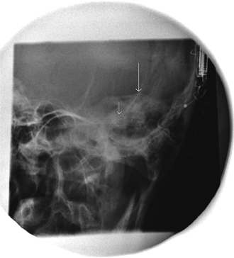
Fig. 1.4 A Stenvers radiograph for cochlear implantation. If the Stenvers radiograph is performed correctly, the cochlear implant lead (short white arrow) should lay coiled in the cochlea, anterior and inferior to the vestibule and lateral and superior semicircular canals (SSCs; summit of SSC marked by long white arrow).
How to protocol the case. You have the requisition in hand. What type of scan do you ask the technologist to do?
How to interpret the study. An interpretive strategy is provided that first considers the clinical background, then highlights the clinical questions most commonly asked by clinicians. Accordingly, a checklist approach to the images is presented.
How to report the findings. A report template is provided to help with the dictation.
Acute Otitis Media
Protocol
A routine CT scan of the temporal bone is the standard protocol.
If there is clinical concern for sinus thrombosis or coalescent mastoiditis, the study is performed with IV contrast. MRI is a more sensitive modality for evaluation of some of the complications of acute otitis media (AOM), such as suppurative labyrinthitis, facial nerve inflammation, and meningitis, but CT is overall the preferred initial study.
Interpretation
Clinical Background
Commonly, patients with AOM present with a bulging ear drum and otalgia and appear sick with fever, malaise, and lethargy. Depending on the level of clinical concern for severity and sequelae of the AOM, the clinician will refer the patient for imaging to evaluate for intratemporal and extratemporal complications of AOM. Long-term antibiotic therapy may be indicated, for instance in the setting of coalescent mastoiditis.8
Clinical Questions
Are there intratemporal (local auricular) complications of AOM, such as coalescent mastoiditis, osseous erosion, facial nerve involvement, or suppurative labyrinthitis?
Are there extratemporal complications of AOM, such as sigmoid sinus thrombosis, epidural abscess, or meningitis?
Approach
Evaluate for evidence of intratemporal complications of AOM.
Inspect the osseous margins of the mastoid for evidence of demineralization (bone algorithm images) and for subperiosteal abscess (soft tissue algorithm images) that may reflect a coalescent mastoiditis. It is our experience that asymmetry of the central trabeculation of the mastoids is not specific for the diagnosis of coalescent mastoiditis and that demineralization along the external or cisternal walls of the sinus is a more reliable sign.
Inspect the osseous margins of the facial nerve canal for demineralization that would suggest inflammatory dehiscence. This evaluation is problematic on CT, as the wall of the tympanic segment is naturally papyraceous. An MRI would be a more sensitive modality for detection of neuritis.
Evaluate for erosion of the walls of the membranous labyrinth that would suggest a suppurative labyrinthitis. Again, an MRI would be a more sensitive modality for evaluation for enhancement of the labyrinth.
Evaluate for a middle ear cavity cholesteatoma.
Evaluate for extratemporal sequelae of AOM.
Inspect the margins of the middle ear cavity (MEC) and mastoid for evidence of epidural or Bezold abscess.
Evaluate the transverse and sigmoid sinus for evidence of thrombosis.
Evaluate the meninges for evidence of meningitis. Here again, an MRI would be a more sensitive modality.
Report
On the right/left, the external auditory canal is severely opacified. The middle ear cavity is completely opacified, and severe periauricular inflammation is noted. There are no findings specific for a coalescent mastoiditis. No erosion is seen along the course of the facial nerve canal or walls of the inner ear. No lobular opacity is seen specific for a cholesteatoma. No extratemporal sequela of acute otitis media is seen: no Bezold or epidural abscess, sinus thrombosis, or meningitis is seen.
Chronic Otitis Media, Chronic Otomastoiditis
Protocol
A noncontrast CT of the temporal bone is the preferred modality.
Interpretation
Clinical Background
Otologists divide patients with chronic otitis media (COM) into three groups:
Active COM with or without cholesteatoma
Inactive COM with retraction pocket, perforation, ossicular resorption, or fixation
Inactive COM with frequent reactivation
The goal of imaging, therefore, is to guide the clinical management (including surgery) in each of these three groups and to evaluate for complications.
Clinical Questions
There are six questions to answer in evaluating a patient with COM. If the radiologist addresses these issues, whatever the group of COM, the major clinical questions will have been answered.
Is there a cholesteatoma, is it confined to the external attic, or has it spread beyond the attic?
Are there any complications of COM, such as perilymphatic or horizontal canal fistulas, tegmen dehiscence, or fallopian canal dehiscence?
Is the mastoid healthy or diseased, and what is the size of the mastoid?
What is the state of the ossicular chain?
Is the external auditory canal (EAC) eroded?
How well aerated is the MEC?
Active Chronic Otitis Media with Cholesteatoma It is important to keep in mind that the radiologist may not sometimes need to make the diagnosis of COM (or sometimes cholesteatoma) if such has been made by the otologist already.
For a patient wth COM and a cholesteatoma, the clinician in his or her consideration of surgical management confers with the radiologist to help answer the following three questions.
Is the cholesteaoma limited to the attic?
Is the mastoid well pneumatized and aerated (healthy) and what is the size of the mastoid?
Is the EAC eroded?
The answers to these questions may lead to three distinct surgical procedures.
If the cholesteatoma is confined to Prussak’s space, and the lateral attic and the mastoid are healthy (well pneumatized and aerated), then an anterior atticotomy may be performed, where the surgeon removes the scutum and lateral attic and leaves the mastoid intact.
If the cholesteatoma extends beyond the attic, and the mastoid is healthy, then a canal wall up (CWU) technique is preferred with a planned second-look procedure.
If the cholesteatoma is beyond the attic, and the mastoid is unhealthy, or if there is erosion of the EAC, then a canal wall down (CWD) technique is preferred.
Other clinical considerations may lead to a CWD technique such as surgical preference, single hearing diseased ear (each surgery carries a 1% risk of sensorineural hearing loss), poor patient compliance, or poor patient health, such that a CWU with second-look would be problematic.
Active Chronic Otitis Media without Cholesteatoma
Stay updated, free articles. Join our Telegram channel

Full access? Get Clinical Tree


