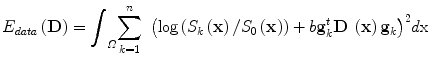
with the tensor D being the unknown variable and b a value that depends on the acquisition settings. The estimation of the tensors in the volume domain Ω can be done through direct inference (6 acquisitions are at least available), which is equivalent to minimizing:
 and Z(x) is a normalization factor, i.e
 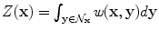 . The most critical aspect of such an approximation model is the definition of weights, measuring the similarity between tensors within the local neighborhood. The use of Gaussian weights is a common weight’s selection, i.e
 ![$$ \left[ {w(\mathbf{x},\mathbf{y}) = {e^{\frac{{ - {d^2}(\mathbf{D}(\mathbf{x}),\mathbf{D}(\mathbf{y}))}}{{2{\sigma ^2}}}}}} \right] $$](/wp-content/uploads/2016/09/A151032_1_En_24_Chapter_IEq3.gif) , where d(.; .) is a distance between tensors and σ a scale factor. In the context of direct estimation and regularization it is more appropriate to define similarities directly on the observation space rather than the estimation space. Such a choice will lead to a tractable estimation, while preserving the convexity of the cost function. Our distance definition as well as our minimization step are based on the representation of symmetric positive semi-definite matrices S +3 as a convex closed cone in the Hilbert space of symmetric matrices S 3, where the standard scalar product is defined by
, where d(.; .) is a distance between tensors and σ a scale factor. In the context of direct estimation and regularization it is more appropriate to define similarities directly on the observation space rather than the estimation space. Such a choice will lead to a tractable estimation, while preserving the convexity of the cost function. Our distance definition as well as our minimization step are based on the representation of symmetric positive semi-definite matrices S +3 as a convex closed cone in the Hilbert space of symmetric matrices S 3, where the standard scalar product is defined by 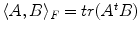 which induces the corresponding Frobenius norm.
3.1 Measuring Similarities from diffusion weighted images
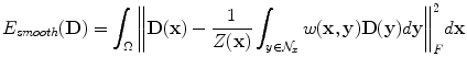
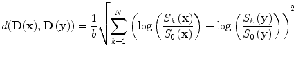
We aim at simultaneously estimating and smoothing the tensor field, therefore the weights w(x, y) in E smooth should be precalculated using the raw data. The most straightforward estimation of the distances can be done through the algebraic distance between the log(S k /S 0) for two neighborhood voxels in any direction
 One can easily show that such an expression does not reflect similarity between tensors according to the norm ∥ ⋅ ∥ F . In fact, this leads to
 such that
 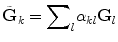 (each new vector of the new basis is a linear combination of the vectors of the initial basis). This procedure allows us to have an approximation of ||D(x) − D(y)|| F directly from the raw data S k and S 0 as follows
![$$ \begin{array}{l}{\parallel}(\mathbf{D}(\mathbf{x})-\mathbf{D}\mathbf{y}){\parallel}_F=\sqrt{{\displaystyle \sum_{k=1}^N<\mathbf{D}\left(\mathbf{x}\right)}-\mathbf{D}\left(\mathbf{y}\right),{\tilde{\mathbf{G}}}_k{>}_F^2}\\ {}\frac{1}{b}=\sqrt{{{\displaystyle \sum_{k=1}^N\left({\displaystyle \sum_l{\alpha}_{k l}\left( \log \left(\frac{S_k\left(\mathbf{x}\right)}{S_0\left(\mathbf{x}\right)}\right)- \log \left(\frac{S_k\left(\mathbf{y}\right)}{S_0\left(\mathbf{y}\right)}\right)\right)}\right)}}^2}\end{array} $$
” src=”/wp-content/uploads/2016/09/A151032_1_En_24_Chapter_Equf.gif”></DIV></DIV></DIV></DIV></DIV><br />
<DIV id=Sec5 class=]()


 Get Clinical Tree app for offline access

such that (each new vector of the new basis is a linear combination of the vectors of the initial basis). This procedure allows us to have an approximation of ||D(x) − D(y)|| F directly from the raw data S k and S 0 as follows3.2 Semi-Definite Positive Gradient Descent
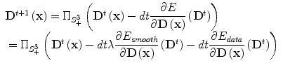
One now can seek the lowest potential of the cost function towards recovering the optimal solution on the tensor space. The present framework consists of a convex energy with a unique minimum which can be reached using a projected gradient descent on the space of semi-definitive positive matrices. The projection from S 3 onto S +3 denoted by  is well defined and has an explicit expression. Indeed, projecting M amounts to replacing the negative eigenvalues in its spectral decomposition by 0 [8, 12]. Note that we minimize over the set of semi-definite positive matrices because it is topologically closed, as opposed to the set of definite positive matrices. In the current setting, the problem is well posed and the projected gradient descent algorithm is convergent for a suitable choice of the time step dt. Using a weighting factor λ between the data attachment term and the regularization energy, the gradient descent can be expressed as the following equation
 where
where
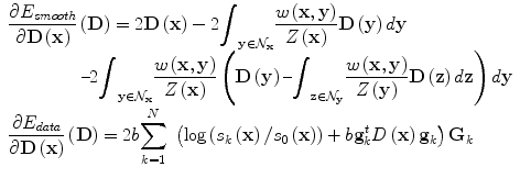
is well defined and has an explicit expression. Indeed, projecting M amounts to replacing the negative eigenvalues in its spectral decomposition by 0 [8, 12]. Note that we minimize over the set of semi-definite positive matrices because it is topologically closed, as opposed to the set of definite positive matrices. In the current setting, the problem is well posed and the projected gradient descent algorithm is convergent for a suitable choice of the time step dt. Using a weighting factor λ between the data attachment term and the regularization energy, the gradient descent can be expressed as the following equationLet us define the norm ∥ ⋅ ∥ TF over the whole tensor field D as ∥ D ∥ TF = ∫ Ω ∥ D(x) ∥ F d x. Considering two tensor fields D 1 and D 2, we show in the following that the gradient of our energy functional is L-Lipschitz. The constant L will allow us to choose automatically a time step that insures the convergence of the algorithm.
 where
where  is the number of the considered neighbors. Thus the gradient of the objective function is L-Lipschitz with
 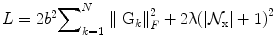 . Choosing
 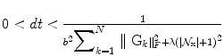 makes the projected gradient descent convergent [3].
is the number of the considered neighbors. Thus the gradient of the objective function is L-Lipschitz with . Choosing makes the projected gradient descent convergent [3].We can give an interpretation of our regularization energy in terms of diffusion-weighted images smoothing. It can be easily verified that for each direction k
![$$ \begin{array}{lll} {\displaystyle\int_\Omega }{ < \mathbf{D}(\mathbf{x}) - \int_{\mathrm{y} \in {{\mathcal N}_\mathrm{x}}} {\dfrac{{{w}(\mathbf{x},\mathbf{y})}}{{Z(\mathbf{x})}}} \mathbf{D}(\mathbf{y})d\mathbf{y},{\mathbf{G}_k}} > _F^2 d\mathbf{x} = \\ \dfrac{1}{{{b^2}}}{\displaystyle\int_\Omega {\left[ {\mathrm{log}\left( {\dfrac{{{S_k}(\mathbf{x})}}{{{S_0}(\mathbf{x})}}} \right) – \mathrm{log} \left( {\prod\limits_{\mathrm{y} \in {{\mathcal N}_\mathrm{x}}} {{{(\dfrac{{{S_k}(\mathbf{y})}}{{{S_0}(\mathbf{y})}})}^{\frac{{\textit{{w}}(\mathrm{x},\mathrm{y})}}{{Z(\mathrm{x})}}}}} } \right)} \right]} ^2}d\mathbf{x} \end{array} $$
” src=”/wp-content/uploads/2016/09/A151032_1_En_24_Chapter_Equk.gif”></DIV></DIV></DIV>Using Cauchy-Schwartz inequality we obtain:<br />
<DIV id=Equl class=Equation><br />
<DIV class=EquationContent><br />
<DIV class=MediaObject><IMG alt=](/wp-content/uploads/2016/09/A151032_1_En_24_Chapter_Equl.gif) We can see that minimizing E smooth has a direct implication on the normalized diffusion weighted images
We can see that minimizing E smooth has a direct implication on the normalized diffusion weighted images  . Reconstructing the tensors using a linear combination of the tensors in its neighborhood leads to the reconstruction of the normalized signals using a weighted geometric mean of the neighboring signals where the weights are not calculated only with a single volume S k but also with the volumes obtained from the other magnetic gradient directions.
. Reconstructing the tensors using a linear combination of the tensors in its neighborhood leads to the reconstruction of the normalized signals using a weighted geometric mean of the neighboring signals where the weights are not calculated only with a single volume S k but also with the volumes obtained from the other magnetic gradient directions.4 SVM classification and kernels on tensors
4.1 Two-class Support Vector Machines
We briefly review the principles of two class SVMs [26]. Given N points x i with known class information y i (either +1 or −1), SVM training consists in finding the optimal separating hyperplane described by the equation w t x + b = 0 with the maximum distance to the training examples. It amounts to solving a dual convex quadratic optimization problem and each data point x is classified using the SVM output function f(x) = (Σ i N α i y i xx i ) + b. The algorithm is extended to achieve non linear separation using a kernel function K(x,y)(symmetric, positive definite) that is used instead of the standard inner product.
4.2 Information diffusion kernel
In order to define a kernel on the set of definite positive matrices, we can propagate class and structure information using its geometry as a Riemannian manifold [22]. Intuitively, we can see the construction of this kernel as diffusing the labels of the training set to the whole set of definite positive matrices. Therefore, similarly to heat diffusion on a Euclidean space, where the solution is given by the convolution of the initial condition by a Gaussian kernel, heat diffusion on a Riemannian manifold is driven by a kernel function K t and given by the following asymptotic series expansion [17]:
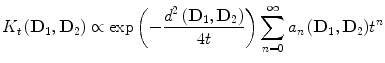 where d corresponds to the geodesic distance induced by the Riemannian metric, a n are the coefficients of the series expansion and t is the diffusion time, which is a parameter of the kernel. We use a first order approximation in t of the previous expression that yields
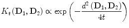 In our case, d has an explicit expression given by
 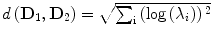 where λ i are the generalized eigenvalues of D 1 and D 2 [22].
where λ i are the generalized eigenvalues of D 1 and D 2 [22].Related posts:

Stay updated, free articles. Join our Telegram channel
Full access? Get Clinical Tree