(1)
where
 are the Fourier transforms at frequency f in channel m for a given segment or trial and
  denotes the expectation value which is typically approximated by an average over the segments or trials.
It is straight forward to show that noninteracting sources do not contribute systematically, i.e. apart from random fluctuations around zero to the imaginary part of the cross-spectra,  , regardless of the number of sources and details of the forward mapping (Nolte et al. 2004). The reason is that the forward mapping is essentially instantaneous and does not induce phase delays to excellent approximation (Stinstra and Peters 1998) which would be necessary to yield a nonvanishing imaginary part of S(f).
 , regardless of the number of sources and details of the forward mapping (Nolte et al. 2004). The reason is that the forward mapping is essentially instantaneous and does not induce phase delays to excellent approximation (Stinstra and Peters 1998) which would be necessary to yield a nonvanishing imaginary part of S(f).
From the cross-spectra S(f) one can construct coherency matrices C(f), which are a normalized version of S(f), as


(2)
In contrast to the imaginary parts of the cross-spectra,  also depends on independent sources through the denominator in Eq. (2). However, independent sources can only lead to a decrease of
  and hence also
  reflects true interaction even though the physiological interpretation is not trivial especially when interpreting differences of
  e.g. between different tasks.
 also depends on independent sources through the denominator in Eq. (2). However, independent sources can only lead to a decrease of
  and hence also
  reflects true interaction even though the physiological interpretation is not trivial especially when interpreting differences of
  e.g. between different tasks.
Based on these observations we suggested a series of methods to identify and localize brain interactions (Nolte et al. 2006; Marzetti et al. 2008; Nolte et al. 2009; Ewald et al. 2012; Shahbazi Avarvand et al. 2012). Additionally, we proposed a method to identify causal structures of the dynamical system under study (Nolte et al. 2008). We here give a brief review of some of these methods (Nolte et al. 2006; Marzetti et al. 2008; Ewald et al. 2012, Shahbazi Avarvand et al. 2012; Nolte et al. 2008) to identify interacting brain sources and to estimate causal relationships. All the methods will be demonstrated using real data whose characteristics are defined in the following section.
2 Data Set
For illustrative purposes, and for illustrative purposes only, we will apply the methods, which will be reviewed throughout this chapter, to an emprirical MEG data set. The data set consists of around 20 min MEG data, under resting state, with 10 min eyes closed and 10 min eyes open. We will average across these two conditions. MEG was measured with a CTF system with 273 channels in Hamburg-Eppendorf.
For the subject an anatomical MRI data set was available which was analyzed with fieldtrip/SPM (Oostenveld et al. 2011) for segmentation to get a volume conductor, which was defined by the inner surface of the skull. Forward calculation was done with an expansion of the magnetic lead field (Nolte 2003).
Spectral analysis was done with a frequency resolution of 0.5 Hz using short-time FFTs of Hanning windowed segments of 2 s duration. In Fig. 1 we show the power for all channels and the imaginary part of coherency (ImCoh) for all pairs of channels as function of frequency. While the peak in the alpha range is very clear it is fairly weak in the beta range and not observable in the gamma range. The rhythms are more clear for ImCoh showing two peaks in the alpha range, at 8 and 10 Hz, a clear peak in the beta range, with a center at 20.5 Hz, and an additional weaker peak at 31 Hz.
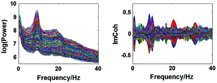

Fig. 1
Power for all channels and ImCoh for all pairs of channels
In general, subjects can be very different. The present subject has prominent peaks of the imaginary part of coherency at alpha, beta, and gamma frequencies both under eyes closed and eyes open condition. The gamma peak is apparently a (second) higher harmonic of the motor alpha rhythm. At the alpha peak the distinction between central and occipital alpha is not straight forward. The beta-peak, on the other hand, appears to be clearly related to activity in sensory-motor areas, which is also the case for the weaker gamma peak. Since we here show just one example for illustration we decided to discuss in the detail the inverse solutions for the beta-rhythm.
In Fig. 2 we show the imaginary part of coherency at 20.5 Hz. Each of the 50 circles represents one out of the total of 273 channels and shows its ImCoh value to all other channels. The subset of 50 equally distributed channels was chosen to ease visibility. We observe clear dipolar structures over both hemispheres, however, with unclear origin from visual inspection.
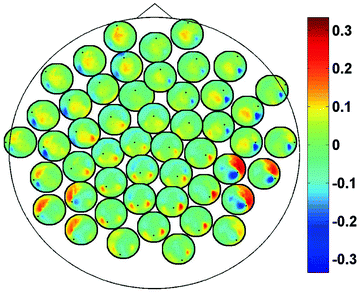

Fig. 2
ImCoh at 20.5 Hz between 50 selected channels and all other channels
3 Methods
3.1 Identifying the Subspace
Below, we will use two different inverse methods to find the sources of the imaginary part of the cross-spectrum. Both methods require the identification of a low dimensional subspace within the channel space. Analogous to the standard PCA decomposition of the full cross-spectrum of a covariance matrix we perform a singular value decomposition of the imaginary part of the cross-spectrum at the signal frequency 


(3)
For some applications it is convenient to estimate a meaningful contrast, i.e. a cross-spectrum which contains similar background noise but not the rhythmic phenomenon which is under study. We will here construct this as an interpolation between neighboring frequencies:


(4)
The singular values of  and the ratios of these and the corresponding singular values of
  are shown in Fig. 3. Since the imaginary parts of cross-spectra are real valued and antisymmetric, all singular values occur in pairs. (For an odd number of channels the last one is zero.) We observe the presence of four prominent singular values. The ratios of singular values converge roughly to
  , indicating that the background noise is estimated too low. This is expected if the background noise consists essentially of non-interacting sources: the linear interpolation effectively doubles the number of averages and since for non-interacting sources the imaginary part of the cross-spectrum drops with
  for N averages, we expect an additional drop by a factor
  . The factor is slightly less than
  which is possibly due to the typical 1/f-decay of the background noise: it is a convex function having the property that linear interpolations are above the true value. Also from this ratio we observe that only 4 singular values are clearly above noise level. In the following we will always analyze this 4-dimensional subspace.
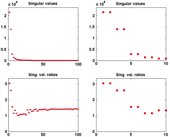
 and the ratios of these and the corresponding singular values of
  are shown in Fig. 3. Since the imaginary parts of cross-spectra are real valued and antisymmetric, all singular values occur in pairs. (For an odd number of channels the last one is zero.) We observe the presence of four prominent singular values. The ratios of singular values converge roughly to
  , indicating that the background noise is estimated too low. This is expected if the background noise consists essentially of non-interacting sources: the linear interpolation effectively doubles the number of averages and since for non-interacting sources the imaginary part of the cross-spectrum drops with
  for N averages, we expect an additional drop by a factor
  . The factor is slightly less than
  which is possibly due to the typical 1/f-decay of the background noise: it is a convex function having the property that linear interpolations are above the true value. Also from this ratio we observe that only 4 singular values are clearly above noise level. In the following we will always analyze this 4-dimensional subspace.
Fig. 3
Top singular values of imaginary part of cross-spectrum at 20.5 Hz. Bottom ratio of singular values of imaginary part of cross-spectrum at 20.5 Hz and a noise cross-spectrum
The singular vectors are shown in Fig. 4. They roughly have dipole structure, but apparently the dipoles are not well separated. A standard method to demix sources is independent component analysis (ICA), which, however, is not appropriate here, since we are studying interacting sources in sharp contrast to the fundamental assumption of ICA. A separation can still be done using dynamical assumptions if one assumes that all interactions are pairwise using the ‘Pairwise Interacting Component Analysis’ (PISA) (Nolte et al. 2006). Then the pairs can be separated from each other but a separation of the two sources within each pair is not possible. Also, for such a separation a wide-band analysis of the data is necessary and cannot be done for a single frequency alone. For completeness, we will sketch the theory behind it, but below we will continue with the space spanned by all chosen singular vectors without dynamical separation.
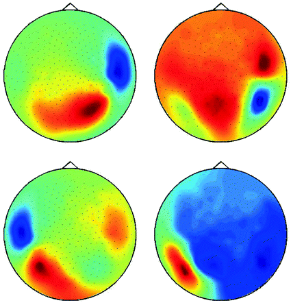

Fig. 4
First four singular vectors of the imaginary of the cross-spectrum at 

In general, EEG and MEG data are a superposition of many subsystems including (effectively) independent sources but also interacting rhythmic sources of various physiological content. To separate these systems one can assume that (a) all interactions are pairwise and that (b) there are not more interacting sources than channels. These two assumptions are a clear simplification of the true brain dynamics, but they yield a unique decomposition of the data and may capture the most relevant aspects of the interaction observed in EEG/MEG data. These assumptions can be expressed for an even number of N channels as a model for the imaginary part of the cross spectra:


(5)
For each k the set of topographies (a k and b k ) and the ‘interaction spectrum’ p k (f) form a—what we call—PISA-component. We note that this model is only unique up to linear mixing of the two topographies for each k. In other words, the model only identifies the 2D-subspace spanned by the two topographies and not the individual components. For technical details we refer to (Nolte et al. 2006).
3.2 Inverse Method
In order to uniquely decompose the 2D-subspaces found by the singular value decomposition into contributions from individual sources we must introduce further spatial constraints on the nature of the sources. To apply a method designed to this purpose, outlined in the next section, it is necessary to use a linear inverse method. While in principle the decomposition in sensor space itself does not depend very much on the chosen inverse method, results in source space can vary substantially. We here use eLORETA (Pascual-Marqui et al. 2011), which is a non-adaptive linear inverse solver with a block-diagonal weight matrix adjusted such that the estimated source distribution has maximal power at the true source for a single dipole. The inverse method will be applied for a predefined grid of voxels in the brain. For the mth brain voxel and for the kth dipole direction and for a given forward model, eLORETA defines a spatial filter G mk , which is a column vector of N elements for N channels, such that for the data vector x(t) in channel space the activity of the kth dipole moment on the mth voxel is given by


(6)
Due to the linearity of the inverse method, one can directly apply the spatial filters to the cross-spectra to estimate the elements of the 3 × 3 cross-spectral matrix P(f, m) at the mth voxel at a given frequency


(7)
The maximum eigenvalue of P(f, m) is the power of the strongest dipole at that location and the corresponding eigenvector is the orientation.
For the present data, the spectral peak in the beta range is very small. Due to the large noise, meaningful source estimates could not be achieved. Instead, it was necessary, to calculate the power in source space both for the S signal and S noise defined in (3) and (4) and to calculate the ratio of powers shown in Fig. 5.2 We observe signal peaks in left and right sensory-motor areas as can be expected for central beta-rhythms. We emphasize that for the estimation of the sources of the interaction, to be conducted in the next section, the localization of power is not necessary, but only serves to demonstrate the consistency of the results.
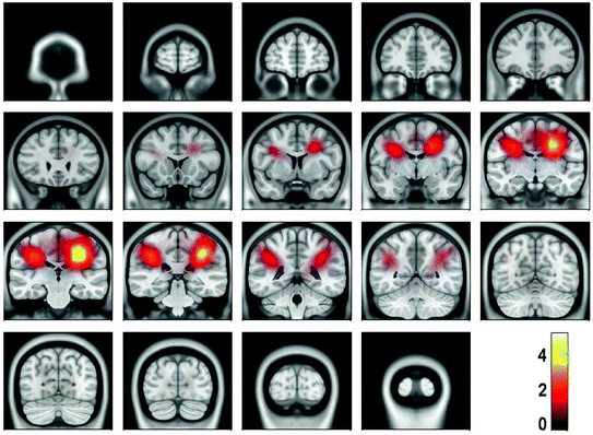

Fig. 5
Power ratio between signal and noise calculated from cross-spectra using eLORETA
3.3 Minimum Overlap Component Analysis
3.3.1 The Concept
The goal of Minimum Overlap Component Analysis (MOCA) is to decompose sets of topographies based on assumptions about the underlying sources and taking note that orthogonality assumptions, as implicit in PCA or SVD decompositions, are unrealistic (Marzetti et al. 2008). We will explain the concept for two topographies. We apply a linear inverse operator G onto the singular vectors x 1 and x 2, such that these topographies are mapped into distributions s i of the source field

where  is a three dimensional vector field calculated in brain voxels
  and in directions
  .
.

(8)
 is a three dimensional vector field calculated in brain voxels
  and in directions
  .
.The distributions do not represent the sources of the brain, denoted as q i , but are, within the accuracy of the inverse method, a yet unknown superposition of them:

for i = 1, 2. The 2 × 2 mixing matrix W can be calculated uniquely under the following constraints

(9)
1.
The sources are orthonormal:

(11)
This cost function first squares the scalar product of two dipole moments at each voxel and then sums these squares over all voxels. It vanishes if the two dipole distributions have disjoint support (i.e. disjoint regions of non-vanishing activity), thus measuring overlap. It also vanishes if the orientations at each voxel are orthogonal and therefore corresponds to a weaker form of overlap allowing in principle also activities at the same location as long as the orientations are sufficiently different. Thus, a strong bias towards remote interaction is removed.
The minimization in Eq. (11) can be done analytically (Marzetti et al. 2008). If the concept is generalized to more than two topographies the minimization requires a numerical approach, which, however, is surprisingly fast and robust (Nolte et al. 2009). We note that the spatial constraints (Eqs. 10, 11) and the methods to solve the minimization are similar to those used in ICA in the context of fMRI data analysis (McKeown and Sejnowski 1998; Matsuda and Yamaguchi 2004) with the major difference that we here decompose vector fields rather than scalar ones. To relate to ICA to decompose EEG and MEG data, the orthogonality constraint in Eq. (10) corresponds, mutatis mutandis, to ‘sphering’ as is used in most ICA methods: the data are transformed to be exactly uncorrelated while independence in higher statistical orders is only forced to be as good as possible.
3.3.2 Illustration
Once the demixing matrix W is found, it can be applied equally to the source distributions and the topographies. If U is an N × K matrix containing the first K singular vectors as columns, and  is the demixing matrix, then
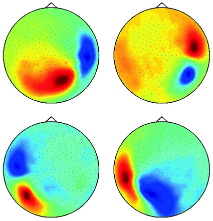
  contains as columns the demixed topographies. The demixed topographies for the singular vectors shown in Fig. 4 are presented in Fig. 6. While, of course, the true result is not known for real data, we observe that the apparent mixture of several dipolar structures has been removed.
 is the demixing matrix, then
  contains as columns the demixed topographies. The demixed topographies for the singular vectors shown in Fig. 4 are presented in Fig. 6. While, of course, the true result is not known for real data, we observe that the apparent mixture of several dipolar structures has been removed.
Fig. 6
Demixed singular vectors using MOCA
In Fig. 7 we show the power of the source estimate for all four demixed topographies. We can see that, similar to the result shown in Fig. 5, sources are located in left and right motor-sensory areas. In contrast to the localization of the entire cross-spectrum, for this localization of the interacting sources it is not necessary to visualize power ratios to achieve meaningful results.
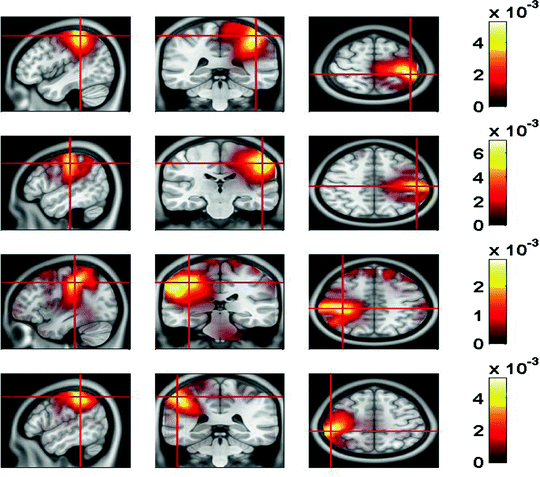

Fig. 7
Sources of demixed singular vectors. Each row displays one source distribution with shown MRI-slices centered at the maximum of the respective power distribution
3.3.3 Minimization of the Cost Function
In this subsection we present the algorithm to solve the minimization problem defined by MOCA. If we only have two source distributions this can be done analytically. To do this we first whiten the distributions s i to fulfill (10


Stay updated, free articles. Join our Telegram channel

Full access? Get Clinical Tree


