TR, TE, and Tissue Contrast
Introduction
In previous chapters, we discussed the roles of T1 and T2, longitudinal and transverse magnetization, and the radio frequency (RF) pulse. Obviously, by doing the procedures described in the previous chapters only once, we won’t be able to create an image. To get any sort of spatial information, the process must be repeated multiple times, as we shall see shortly. This is where TR and TE come into play. The parameters TR and TE are related intimately to the tissue parameters T1 and T2, respectively. However, unlike T1 and T2, which are inherent properties of the tissue and therefore fixed, TR and TE can be controlled and adjusted by the operator. In fact, as we shall see later, by appropriate setting of TR and TE, we can put more “weight” on T1 or T2, depending on the type of clinical application.
How do we actually measure a signal? With the patient in a large magnetic field (Fig. 5-1A), we apply a 90° RF pulse, and the magnetization vector flips into the x-y plane (Fig. 5-1B). Then, we turn off the 90° RF pulse, and the magnetization vector begins to grow in the z direction and decay in the x-y plane (Fig. 5-1C). By convention, we apply the RF pulse in the x direction, and for that reason, in a rotating frame of reference, the vector ends up along the y-axis (Fig. 5-1B).
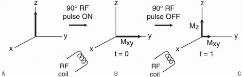 |
After a 90° RF pulse, we have decaying transverse magnetization Mxy (which is the component of the magnetization vector in the x-y plane) and recovering longitudinal magnetization Mz (which is the component of the magnetization vector along the z-axis). Remember that the received signal can be detected only along the x-axis, that is, along the direction of the RF transmitter/receiver coil. The receiver coil only recognizes oscillating signals (like AC voltage) and not nonoscillating voltage changes (like DC voltage). Thus, rotation in the x-y plane induces a signal in the RF coil, whereas changes along the z-axis do not.
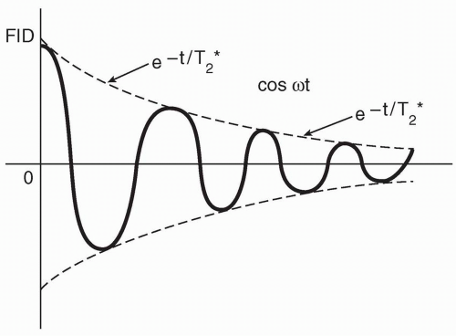 Figure 5-2. The received signal (the FID) has a decaying sinusoidal waveform. |
At time t = 0, the signal is at a maximum. As time goes by, because of dephasing (see Chapter 4), the signal becomes weaker in a sinusoidal manner (Fig. 5-2). The decay curve of the signal is given by the following term: e−t/T2*
The sinusoidal nature of the signal is given by the equation cos ωt
When t = 0, (e−t/T2*)(cos ωt) = 1. Thus, at time t = 0, the signal is maximum (i.e., 100%). As time increases, we are multiplying a sinusoidal function (cos ωt) and a decaying function (e−t/T2*), which eventually decays to zero (Fig. 5-3).
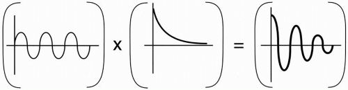 Figure 5-3. The product of a sinusoidal signal and an exponentially decaying signal results in a decaying sinusoidal signal. |
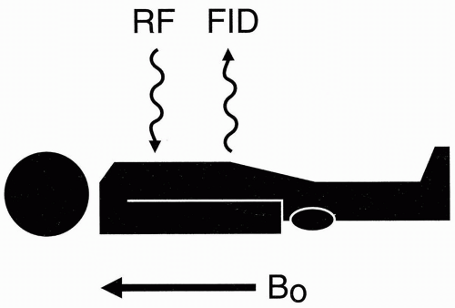
When we put a patient in a magnet, he or she becomes temporarily magnetized as his or her protons align with the external magnetic field along the z-axis. We then transmit an RF pulse at the Larmor frequency and immediately get back a free induction decay (FID; Fig. 5-4). This process gives one signal—one FID—from the entire patient. It doesn’t give us any information about the location of the signal. The FID is received from the ensemble of all the different protons in the patient’s body with no spatial discrimination. To get spatial information, we have to specify somehow the x, y, and z coordinates of the signal. Here, gradients come into play. The purpose of the gradient coils is to spatially encode the signal.
To spatially encode the signal, we have to apply the RF pulse multiple times while varying the gradients and, in turn, get multiple FIDs or other signals (e.g., spin echoes). When we put all the information from the multiple FIDs together, we get the information necessary to create an image. If we just apply the RF pulse once, we only get one signal (one FID), and we
cannot make an image from one signal. (An exception to this statement is echoplanar imaging [EPI], which is performed after one RF pulse—see Chapter 22.)
cannot make an image from one signal. (An exception to this statement is echoplanar imaging [EPI], which is performed after one RF pulse—see Chapter 22.)
TR (The Repetition Time)
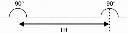
After we apply one 90° pulse (the symbol we’ll use for a 90° RF pulse is in Fig. 5-5), we’ll apply another. The time interval between applications is called TR (the repetition time).
Immediately before time t = 0, the magnetization vector points along the z-axis. Call this vector M0 with magnitude M0.
Immediately after t = 0, the magnetization vector Mxy lies in the x-y plane, without a component along the z-axis. Mxy has magnitude M0 at t = 0+.
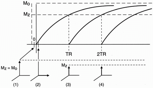
Figure 5-6. The recovery curves after successive RF pulses.
As time goes by and we reach time t = TR, we gradually recover some magnetization along the z-axis and lose some (or all) magnetization in the x-y plane. Let’s assume at time TR the transverse magnetization Mxy is very small. What happens if we now apply another 90° RF pulse? We flip the existing longitudinal magnetization vector (Mz) back into the x-y plane. However, what is the magnitude of the magnetization vector Mz at the time TR? Because Mz(t) = M0(1 − e−t/T1) then at t = TR,

As we see in the T1 recovery curve, the magnetization vector (Mz) at time TR is less than the original magnetization vector M0 because the second 90° RF pulse was applied before complete recovery of the magnetization vector Mz.
Received Signal
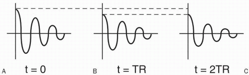
Let’s now take a look at the signal we are receiving (S). Because we are only applying a series of 90° pulses, the signal will be a series of FIDs:
Because the T1 recovery curve is given by the formula 1 − e−t/T1, if we could measure the signal immediately after the RF pulse is given with no delay, then each FID signal would be proportional to 1 − e−TR/T1
(This cannot really happen in practice.) Up to now, the signal S is given by the formula S ∝ 1 − e−TR/T1
Remember that the word “signal” is really a relative term. The signal that we get is a number without dimension, that is, it has no units. If we are dealing with a tissue that has many mobile protons, then, regardless of what the TR and T1 of the tissue are, we’ll get more signals with more mobile protons (see Chapter 2). Thus, when considering the signal, we must also consider the number of mobile protons N(H).
For a given tissue, the T1 and the proton density are constant, and the signal received will be according to the above formula. If we measure the FID at time TR immediately after the application of the second 90° RF pulse, it will measure maximal and be equal to N(H) (1 − e−TR/T1). Therefore, the FIDs that are acquired at TR intervals (i.e., 1TR, 2TR) are maximal if they can be measured right after the 90° pulse, that is, right at the beginning of the FID. However, in reality, we have to wait a certain period until the system electronics allows us to make a measurement.
TE (Echo Delay Time or Time to Echo)
TE stands for echo delay time (or time to echo). Instead of making the measurement immediately after the RF pulse (which we could not do anyway), we wait a short period of time and then make the measurement. This short time period is referred to as TE.
Let’s go back to the T2*


Related posts:
Stay updated, free articles. Join our Telegram channel
Full access? Get Clinical Tree
