Treatment Planning II: Patient Data Acquisition, Treatment Verification, and Inhomogeneity Corrections

Basic depth dose data and isodose curves are usually measured in a cubic water phantom having dimensions much larger than the field sizes used clinically. Phantom irradiations for this purpose are carried out under standard conditions, for example, beams incident normally on the flat surface at specified distances. The patient’s body, however, is neither homogeneous nor flat in surface contour. Thus, the dose distribution in a patient may differ significantly from the standard distribution. This chapter discusses several aspects of treatment planning, including acquisition of patient data, correction for contour curvature, and tissue inhomogeneities and patient positioning.

12.1. ACQUISITION OF PATIENT DATA

Accurate patient dosimetry is only possible when sufficiently accurate patient data are available. Such data include body contour outline, density of relevant internal structures, and location and extent of the target volume. Acquisition of these data is necessary whether the dosimetric calculations are performed manually or with a computer. However, this important aspect of treatment planning is often executed poorly. For example, in a busy department there may be an inordinate amount of pressure to begin the patient’s treatment without adequate dosimetric planning. In other cases, lack of sufficient physics support and/or equipment is the cause of this problem. In such a case, it must be realized that the final accuracy of the treatment plan is strongly dependent on the availability of the patient data and that great effort is needed to improve its quality.

A. BODY CONTOURS

Acquisition of body contours and internal structures is best accomplished by 3-D volumetric imaging [computed tomography (CT), magnetic resonance imaging (MRI), etc.]. The scans are performed specifically for treatment-planning purposes, with the patient positioned the same way as for actual treatment. In 3-D treatment planning (Chapter 19), these data are all image based and are acquired as part of the treatment-planning process. However, for cases in which 3-D treatment planning is not considered necessary or if body contours are obtained manually for verification of the image-based contours, mechanical or electromechanical methods are used for contouring.

A number of devices have been made to obtain patient contours. Some of these are commercially available, while others can be fabricated in the department machine shop. The most common and the simplest of the devices used in the early days of radiotherapy was a solder wire or a lead wire embedded in plastic. Because the wire did not faithfully retain the contour dimensions when transferring it from the patient to the paper, it was necessary to independently measure anteroposterior (AP) and/or lateral diameters of the contour with a caliper.

Another one of the early mechanical devices (1) consisted of an array of rods, the tips of which were made to touch the patient’s skin and then placed on a sheet of paper for contour drawing. Perhaps the most accurate of the mechanical devices is a pantograph-type apparatus
(Fig. 12.1) in which a rod can be moved laterally as well as up and down. When the rod is moved over the patient contour, its motion is followed by a pen that records the outline on paper.

Figure 12.1. Photograph of a contour plotter. (Courtesy of Radiation Products Design, Buffalo, MN.) [Source: www.rpdinc.com.]

Although any of the above methods can be used with sufficient accuracy if carefully used, some important points must be considered in regard to manual contour making:

The patient contour must be obtained with the patient in the same position as used in the actual treatment. For this reason, probably the best place for obtaining the contour information is with the patient properly positioned on the treatment simulator couch.
A line representing the tabletop must be indicated in the contour so that this horizontal line can be used as a reference for beam angles.
Important bony landmarks as well as beam entry points, if available, must be indicated on the contour.
Checks of body contour are recommended during the treatment course if the contour is expected to change due to a reduction of tumor volume or a change in patient weight.
If body thickness varies significantly within the treatment field, contours should be determined in more than one plane.

B. INTERNAL STRUCTURES

Localization of internal structures for treatment planning should provide quantitative information in regard to the size and location of critical organs and inhomogeneities. Although qualitative information can be obtained from diagnostic radiographs or atlases of cross-sectional anatomy, they cannot be used directly for precise localization of organs relative to the external contour. In order for the contour and the internal structure data to be realistic for a given patient, the localization must be obtained under conditions similar to those of the actual treatment position and on a couch similar to the treatment couch.

The following devices are used in modern times for the localization of internal structures and the target volume. A brief discussion regarding their operation and function will be presented.

B.1. Computed Tomography

In CT, a narrow beam of x-rays scans across a patient in synchrony with a radiation detector on the opposite side of the patient. If a sufficient number of transmission measurements are taken at different orientations of the x-ray source and detector (Fig. 12.2A), the distribution of attenuation coefficients within the layer may be determined. By assigning different levels to different attenuation coefficients, an image can be reconstructed that represents various structures with different attenuation properties. Such a representation of attenuation coefficients constitutes a CT image.

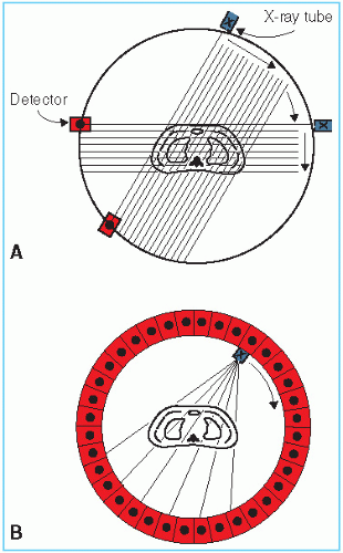Figure 12.2. Illustration of scan motions in computed tomography. A: An early design in which the x-ray source and the detector performed a combination of translational and rotational motion. B: A modern scanner in which the x-ray tube rotates within a stationary circular array of detectors.

Since CT scanning was introduced about 40 years ago, there has been a rapid development in both the software and hardware. Most of the improvements in hardware had to do with the scanner motion and the multiplicity of detectors to decrease the scan time. Figure 12.2B illustrates a modern scanner in which the x-ray tube rotates within a circular array of 1,000 or more detectors. With such scanners, scan times as fast as 1 second or less are achievable. Figure 12.3 shows a typical CT image.

In a slice-by-slice CT scanner, the x-ray tube rotates around the patient to image one slice at a time. In a spiral or helical CT scanner, the x-ray tube spins axially around the patient while the patient is translated longitudinally through the scanner aperture. In such a scanner, multiple detector rings are in place to scan several slices during each gantry rotation.

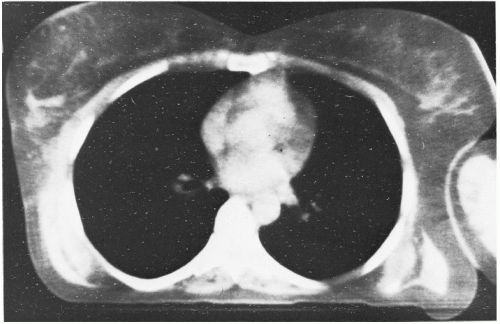Figure 12.3. Typical computed tomography image.

Reconstruction of an image by CT is a mathematical process of considerable complexity, performed by a computer. For a review of various mathematical approaches for image reconstruction, the reader is referred to a paper by Brooks and Di Chiro (2). The reconstruction algorithm divides each axial plane into small voxels, and generates what is known as CT numbers, which are related to calculated attenuation coefficient for each voxel. Typically CT numbers start at -1,000 for vacuum and pass through 0 for water. The CT numbers normalized in this manner are called Hounsfield numbers (H):

where µ is the linear attenuation coefficient. Thus, a Hounsfield unit represents a change of 0.1 % in the attenuation coefficient of water. The Hounsfield numbers for most tissues are close to 0, and approximately +1,000 for bone, depending on the bone type and energy of the CT beam.

Because the CT numbers bear a linear relationship with the attenuation coefficients, it is possible to infer electron density (electrons cm^–³) as shown in Figure 12.4. Although CT numbers can be correlated with electron density, the relationship is not linear in the entire range of tissue densities. The nonlinearity is caused by the change in atomic number of tissues, which affects the proportion of beam attenuation by Compton versus photoelectric interactions. Figure 12.4 shows a relationship that is linear between lung and soft tissue but nonlinear between soft tissue and bone. In practice, the correlation between CT numbers and electron density of various tissues can be established by scanning phantoms of known electron densities in the range that includes lung, muscle, and bone.

Atomic number information can also be obtained if attenuation coefficients are measured at two different x-ray energies (3). It is possible to transform the attenuation coefficients measured by CT at diagnostic energies to therapeutic energies (4). However, for low-atomic-number materials such as fat, air, lung, and muscle, this transformation is not necessary for the purpose of calculating dose distributions and inhomogeneity corrections (4).

Although external contour and internal structures are well delineated by CT, their use in treatment planning requires that they be localized accurately with respect to the treatment geometry. Diagnostic CT scans obtained typically on a curved tabletop with patient position different from that to be used in treatment have limited usefulness in designing technique and dose distribution.
Special treatment-planning CT scans are required with full attention to patient positioning and other details affecting treatment parameters.

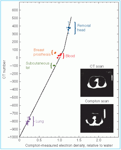Figure 12.4. Computed tomography (CT) numbers plotted as a function of electron density relative to water. (From Battista JJ, Rider WD, Van Dyk J. Computed tomography for radiotherapy planning. Int J Radiat Oncol Biol Phys. 1980;6:99, with permission.)

Some of the common considerations in obtaining treatment-planning CT scans are the following: (a) a flat tabletop should be used; usually a flat carbon fiber overlay which closely mirrors the treatment couch is mounted in the CT cradle; (b) a large-diameter CT aperture (e.g., ≥70 cm) can be used to accommodate unusual arm positions and other body configurations encountered in radiation therapy; (c) care should be taken to use patient-positioning or immobilization devices that do not cause image artifacts; (d) patient positioning, leveling, and immobilization should be done in accordance with the expected treatment technique or simulation if done before CT; (e) external contour landmarks can be delineated using radiopaque markers such as plastic catheters; and (f) image scale should be accurate both in the X and Y directions.

B.2. Three-Dimensional Treatment Planning

Additional considerations go into CT scanning for 3-D treatment planning. Because the 3-D anatomy is derived from individual transverse scans (which are imaged in 2-D), the interslice distance must be sufficiently small to accurately reconstruct the image in three dimensions. Depending on the tumor site or the extent of contemplated treatment volume, contiguous scans are taken with slice thickness ranging from 1 to 10 mm. The total number of slices may range from 30 to over 100. This requires fast scan capability to avoid patient movement or discomfort.

Delineation of target and critical organs on each of the scans is necessary for the 3-D reconstruction of these structures. This is an extremely time-consuming procedure, which has been a deterrent to the adoption of 3-D treatment planning on a routine basis. Efforts have been directed toward making this process less cumbersome such as automatic contouring, pattern recognition, and other computer manipulations. However, the basic problem remains that target delineation is inherently a manual process. Although radiographically visible tumor boundaries can be recognized by appropriate computer software, the extent of target volume depends on grade, stage, and patterns of tumor spread to the surrounding structures. Clinical judgment is required in defining the target volume. Obviously, a computer cannot replace the radiation oncologist! At least, not yet.

Besides the time-consuming process of target localization, 3-D computation of dose distribution and display requires much more powerful computers in terms of speed and storage capacity than the conventional treatment-planning systems. However, with the phenomenal growth of computer technology, this is not perceived to be a significant barrier to the adoption of routine 3-D planning.

3-D planning has already been found to be useful and practical for most tumors or tumor sites (e.g., head and neck, lung, prostrate). Treatment of well-localized small lesions (e.g., <4 cm in diameter) in the brain or close to critical structures by stereotactic radiosurgery has greatly benefited from 3-D planning. In this procedure, the target volume is usually based on the extent of visible tumor (i.e., with CT and/or MR imaging), thus obviating the need for manual target delineation on each CT slice. The 3-D display of dose distribution to assess coverage of the target volume confined to a relatively small number of slices is both useful and practical. Similarly, brachytherapy is amenable to 3-D planning because of the limited number of slices involving the target.

Treatment-planning software is available whereby margins around the target volume can be specified to set the field boundaries. After optimizing field margins, beam angles, and other plan parameters, the dose distributions can be viewed in other slices either individually or simultaneously by serial display on the screen. Beam’s eye view (BEV) display in which the plan is viewed from the vantage point of the radiation source (in a plane perpendicular to the central axis) is useful in providing the same perspective as a simulator or port film. In addition, a BEV outline of the field can be obtained to aid in the design of custom blocks for the field. More discussion on CT-based treatment planning is provided in Chapter 19.

B.3. Magnetic Resonance Imaging

MRI has developed, in parallel to CT, into a powerful imaging modality. Like CT, it provides anatomic images in multiple planes. Whereas CT provides basically transverse axial images (which can be further processed to reconstruct images in other planes or in three dimensions), MRI can be used to scan directly in axial, sagittal, coronal, or oblique planes. This makes it possible to obtain optimal views to enhance diagnostic interpretation or target delineation for radiotherapy. Other advantages over CT include not involving the use of ionizing radiation, higher contrast, and better imaging of soft tissue tumors. Some disadvantages compared with CT include lower spatial resolution; inability to image bone or calcifications; longer scan acquisition time, thereby
increasing the possibility of motion artifacts; and magnetic interference with metallic objects. The above cursory comparison between CT and MRI shows that the two types of imaging are complementary.

Basic physics of MRI involves a phenomenon known as nuclear magnetic resonance (NMR). It is a resonance transition between nuclear spin states of certain atomic nuclei when subjected to a radiofrequency (RF) signal of a specific frequency in the presence of an external magnetic field. The nuclei that participate in this phenomenon are the ones that intrinsically possess spinning motion (i.e., have angular momentum). These rotating charges act as tiny magnets with associated magnetic dipole moment, a property that gives a measure of how quickly the magnet will align itself along an external magnetic field. Because of the spinning motion or the magnetic dipole moment, nuclei align their spin axes along the external magnetic field (H) as well as orbit or precess around it (Fig. 12.5). The frequency of precession is called the Larmor frequency. A second alternating field is generated by applying an alternating voltage (at the Larmor frequency) to an RF coil. This field is applied perpendicular to H and rotates around H at the Larmor frequency. This causes the nuclei to precess around the new field in the transverse direction. When the RF signal is turned off, the nuclei return to their original alignment around H.
This transition is called relaxation. It induces a signal in the receiving RF coil (tuned to the Larmor frequency), which constitutes the NMR signal.

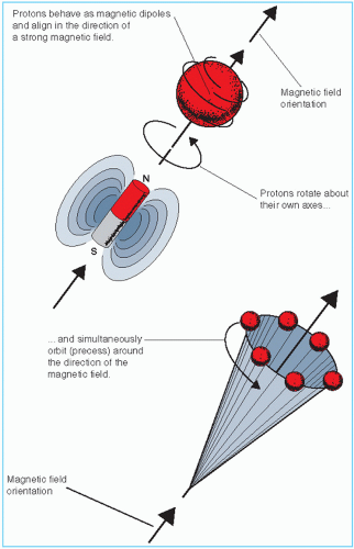Figure 12.5. Alignment and precession of protons in a strong magnetic field. (From Halverson RA, Griffiths HJ, Lee BCP, et al. Magnetic resonance imaging and computed tomography in the determination of tumor and treatment volume. In: Levitt SH, Khan FM, Potish RA, eds. Technological Basis of Radiation Therapy. 2nd ed. Philadelphia, PA: Lea & Febiger; 1992:38, with permission.)

The turning off of the transverse RF field causes nuclei to relax in the transverse direction (T₂ relaxation) as well as to return to the original longitudinal direction of the magnetic field (T₁ relaxation). This is schematically illustrated in Figure 12.6. The relaxation times, T₁ and T₂, are actually time constants (like the decay constant in radioactive decay) for the exponential function that governs the two transitions.

The signal source in MRI can be any nucleus with nonzero spin or angular momentum. However, certain nuclei give larger signal than the others. Hydrogen nuclei (protons), because of their high intrinsic sensitivity and high concentration in tissues, produce signals of sufficient strength for imaging. Other possible candidates are ³¹P, ²³Na, ¹⁹F, ¹³C, and ²H. Most routine MRI is based exclusively on proton density and proton relaxation characteristics of different tissues.

Localization of protons in a 3-D space is achieved by applying magnetic field gradients produced by gradient RF coils in three orthogonal planes. This changes the precession frequency of protons spatially, because the MR frequency is linearly proportional to field strength. Thus, by the appropriate interplay of the external magnetic field and the RF field gradients, proton
distribution can be localized. A body slice is imaged by applying field gradient along the axis of the slice and selecting a frequency range for readout. The strength of the field gradient determines the thickness of the slice (the greater the gradient, the thinner the slice). Localization within the slice is accomplished by phase encoding (using back-to-front Y gradient) and frequency encoding (using transverse X gradient). In the process, the computer stores phase (angle of precession of the proton at a particular time) and frequency information and reconstructs the image by mathematical manipulation of the data.

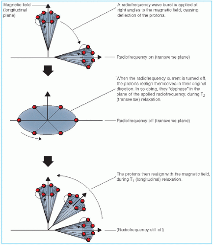Figure 12.6. Effects of radiofrequency applied at right angles to the magnetic field. (From Halverson RA, Griffiths HJ, Lee BCP, et al. Magnetic resonance imaging and computed tomography in the determination of tumor and treatment volume. In: Levitt SH, Khan FM, Potish RA, eds. Technological Basis of Radiation Therapy. 2nd ed. Philadelphia, PA: Lea & Febiger; 1992:38, with permission.)

Most MR imaging uses a spin echo technique in which a 180-degree RF pulse is applied after the initial 90-degree pulse and the resulting signal is received at a time that is equal to twice the interval between the two pulses. This time is called the echo time (TE). The time between each 90-degree pulse in an imaging sequence is called the repetition time (TR). By adjusting TR and TE, image contrast can be affected. For example, a long TR and short TE produces a proton (spin) density-weighted image, a short TR and a short TE produces a T₁-weighted image, and a long TR and a long TE produces a T₂-weighted image. Thus, differences in proton density, T₁, and T₂ between different tissues can be enhanced by a manipulation of TE and TR in the spin echo technique.

Figure 12.7 shows examples of MR images obtained in the axial, sagittal, and coronal planes. By convention, a strong MR signal is displayed as white and a weak signal is displayed as dark on the cathode ray tube (CRT) or film.

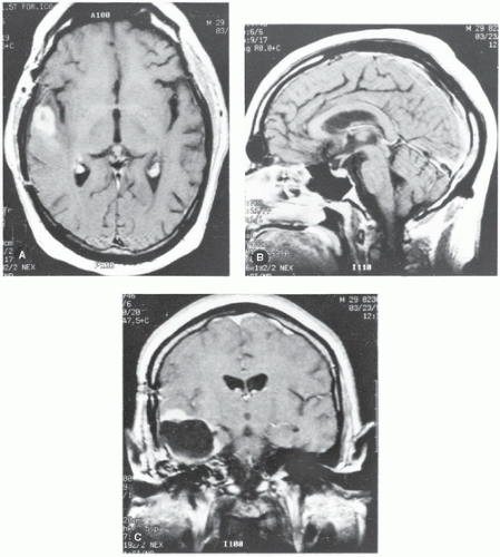Figure 12.7. Examples of magnetic resonance images of the head. A: Transverse plane. B: Sagittal plane. C: Coronal plane.

FUNCTIONAL MAGNETIC RESONANCE IMAGING. Functional magnetic resonance (fMRI) is a technique that detects changes in blood flow in the brain, thereby providing information on brain activity. When neuronal activity increases in a region of the brain, there is an increased demand for oxygen. This in turn stimulates a localized increase in blood flow as well as expansion of the blood vessels. Increased blood flow brings in more oxygen in the form of oxygenated hemoglobin molecules in red blood cells. Because hemoglobin is diamagnetic (slightly repelled by magnetic field) when oxygenated and paramagnetic (slightly attracted by magnetic field) when deoxygenated, the MR signal of blood varies depending on the degree of oxygenation. This form of MRI is also called BOLD (blood oxygen level dependent) imaging. BOLD is the source of contrast in fMRI.

Functional MRI is being used extensively in the study of brain function and has found many applications in the field of cognitive neuroscience. It can also be useful in radiotherapy treatment planning to avoid irradiating critical functional regions at risk in the brain (5, 6, 7).

MAGNETIC RESONANCE SPECTROSCOPY IMAGING. Magnetic resonance spectroscopy (MRS) is a technique that allows the study of metabolic changes in various tissues of the body. The MRS equipment is used to detect and analyze signals from a number of chemical nuclei such as hydrogen, carbon, phosphorus, sodium, and fluorine. This capability allows the study of metabolites by analyzing different peaks in the MR spectrum. The biochemical information thus obtained can be used to diagnose diseases or characterize tumors. In radiation therapy, MRS imaging has been used to characterize prostate and brain tumors (8,9).

B.4. Ultrasound

Ultrasonic imaging for delineating patient contours and internal structures is recognized as an important tool in radiation therapy. Tomographic views provide cross-sectional information that is helpful for treatment planning. Although in most cases the image quality or clinical reliability is not as good as that of CT, ultrasonic procedure does not involve ionizing radiation, is less expensive, and in some cases, yields data of comparable usefulness.

Ultrasound can provide useful information in localizing many malignancy-prone structures in the lower pelvis, retroperitoneum, upper abdomen, breast, and chest wall (10,11). Ultrasound is also used in localization of prostate for image-guided radiation therapy (Chapter 25). The most common application of ultrasound in radiotherapy, however, is the delineation of the prostate for ultrasound-guided prostate implants (Chapter 23).

An ultrasound (or ultrasonic) wave is a sound wave having a frequency greater than 20,000 cycles per second or hertz (Hz). At this frequency, the sound is inaudible to the human ear. Ultrasound waves of frequencies 1 to 20 MHz are used in diagnostic radiology.

Ultrasound may be used to produce images either by means of transmission or reflection. However, in most clinical applications, use is made of ultrasonic waves reflected from different tissue interfaces. These reflections or echoes are caused by variations in acoustic impedance of materials on opposite sides of the interfaces. The acoustic impedance (Z) of a medium is defined as the product of the density of the medium and the velocity of ultrasound in the medium. The larger the difference in Z between the two media, the greater is the fraction of ultrasound energy reflected at the interface. For example, strong reflections of ultrasound occur at the air-tissue, tissue-bone, and chest wall-lung interfaces due to high impedance mismatch. However, because lung contains millions of air-tissue interfaces, strong reflections at the numerous interfaces prevent its use in lung imaging.

Attenuation of the ultrasound by the medium also plays an important role in ultrasound imaging. This attenuation takes place as the energy is removed from the beam by absorption, scattering, and reflection. The energy remaining in the beam decreases approximately exponentially with the depth of penetration into the medium, allowing attenuation in different media to be characterized by attenuation coefficients. As the attenuation coefficient of ultrasound is very high for bone compared with soft tissue, together with the large reflection coefficient of a tissue-bone interface, it is difficult to visualize structures lying beyond bone. On the other hand, water, blood, fat, and muscle are very good transmitters of ultrasound energy.

Ultrasonic waves are generated as well as detected by an ultrasonic probe or transducer. A transducer is a device that converts one form of energy into another. An ultrasonic transducer converts electrical energy into ultrasound energy, and vice versa. This is accomplished by a process known as the piezoelectric effect. This effect is exhibited by certain crystals in which a variation of an electric field across the crystal causes it to oscillate mechanically, thus generating acoustic waves. Conversely, pressure variations across a piezoelectric material (in response to an incident ultrasound wave) result in a varying electrical potential across opposite surfaces of the crystal.

Figure 12.8. Ultrasonic tomogram showing chest wall thickness (right) compared with the computed tomography image (left).

Although the piezoelectric effect is exhibited by a number of naturally occurring crystals, most common crystals used clinically are made artificially such as barium titanate, lead zirconium titanate, and lead metaniobate. The piezoelectric effect produced by these materials is mediated by their electric dipole moment, the magnitude of which can be varied by addition of suitable impurities.

As the ultrasound wave reflected from tissue interfaces is received by the transducer, voltage pulses are produced that are processed and displayed on the CRT, usually in one of three display modes: A (amplitude) mode, B (brightness) mode, and M (motion) mode. A mode consists of displaying the signal amplitude on the ordinate and time on the abscissa. The time, in this case, is related to distance or tissue depth, given the speed of sound in the medium. In the B mode, a signal from a point in the medium is displayed by an echo dot on the CRT. The (x, y) position of the dot on the CRT indicates the location of the reflecting point at the interface and its proportional brightness reveals the amplitude of the echo. By scanning across the patient, the B-mode viewer sees an apparent cross section through the patient. Such cross-sectional images are called ultrasonic tomograms.

In the M mode of presentation, the ultrasound images display the motion of internal structures of the patient’s anatomy. The most frequent application of M-mode scanning is echocardiography. In radiotherapy, the cross-sectional information used for treatment planning is exclusively derived from the B-scan images (Fig. 12.8).

12.2. TREATMENT SIMULATION

A. RADIOGRAPHIC SIMULATOR

Treatment simulator (Fig. 12.9) is an apparatus that uses a diagnostic x-ray tube but duplicates a radiation treatment unit in terms of its geometric, mechanical, and optical properties. The main function of a simulator is to display the treatment fields so that the target volume may be accurately encompassed without delivering excessive irradiation to surrounding normal tissues. By radiographic visualization of internal organs, correct positioning of fields and shielding blocks can be obtained in relation to external landmarks. Most commercially available simulators have fluoroscopic capability by dynamic visualization before a hard copy is obtained in terms of the simulator radiography.

The need for simulators arises from four facts: (a) geometric relationship between the radiation beam and the external and internal anatomy of the patient cannot be duplicated by an ordinary diagnostic x-ray unit; (b) although field localization can be achieved directly with a therapy machine by taking a port film, the radiographic quality is poor because of very high beam energy, and for cobalt-60, a large source size as well; (c) field localization is a time-consuming process that, if carried out in the treatment room, could engage a therapy machine for a prohibitive length of time; and (d) unforeseen problems with a patient setup or treatment technique can be solved during simulation, thus conserving time within the treatment room.

Although the practical use of simulators varies widely from institution to institution, the simulator room has assumed the role of a treatment-planning room. Besides localizing treatment volume and setting up fields, other necessary data can also be obtained at the time of simulation. Because the simulator table is supposed to be similar to the treatment table, various patient measurements such as contours and thicknesses, including those related to compensator or bolus design, can be obtained under appropriate setup conditions. Fabrication of immobilization
devices and testing of individualized shielding blocks can also be accomplished with a simulator. To facilitate such measurements, simulators are equipped with accessories such as laser lights, contour maker, and shadow tray.

Figure 12.9. A: Photograph of Varian Ximatron CDX simulator at the University of Minnesota. B: Varian Acuity simulator that has superseded the Ximatron. (Courtesy of Varian Associates, Palo Alto, CA.)

Modern simulators combine the capabilities of radiographic simulation, planning, and verification in one system. These systems provide commonality in hardware and software of the treatment machine including 2-D and 3-D imaging, accessory mounts, treatment couch, and multileaf collimator (MLC). One such system is Acuity (Varian Medical Systems, Palo Alto, CA) (Fig. 12.9B).

Due to the need for CT image data for the increased role of CT-based treatment planning, the conventional treatment simulator has largely been replaced by the CT Simulator.

B. CT SIMULATOR

An important development in the area of simulation has been that of converting a CT scanner into a simulator. CT simulation uses a CT scanner to localize the treatment fields on the basis of the patient’s CT scans. A computer program, specifically written for simulation, automatically positions the patient couch and the laser cross-hairs to define the scans and the treatment fields. The software (as part of CT scanner or a stand-alone treatment-planning system) provides outlining of external contours, target volumes and critical structures, interactive portal displays and placement, review of multiple treatment plans, and a display of isodose distribution. This process is known as virtual simulation.

The nomenclature of virtual simulation arises out of the fact that both the patient and the treatment machine are virtual—the patient is represented by CT images and the treatment machine is modeled by its beam geometry and expected dose distribution. The simulation film in this case is a reconstructed image called the DRR (digitally reconstructed radiograph), which has the appearance of a standard 2-D simulation radiograph but is actually generated from CT scan data by mapping average CT values computed along ray lines drawn from a “virtual source” of radiation to the location of a “virtual film.” DRR is essentially a calculated (i.e., computer-generated) port film that serves as a simulation film. The quality of the anatomic image is not as good as the simulation radiograph but it contains additional useful information such as the outlined target area, critical structures, and beam aperture defined by blocks or MLC. Figure 12.10 shows an anterior field DRR (A) and a posterior oblique field DRR (B). A DRR can substitute for a simulator radiograph by itself, but it is always preferable to obtain final verification by comparing it with a radiographic simulation film.

Figure 12.10. A: Digitally reconstructed radiograph (DRR) anterior field. B: DRR posterior oblique.

A dedicated radiation therapy CT scanner with simulation accessories (e.g., flat table, laser lights for positioning, immobilization and image registration devices, and appropriate software for virtual simulation) is called a CT simulator. Many types of such units are commercially available. Figure 12.11 shows one example.

C. PET/CT

Positron emission tomography (PET) provides functional images that can, in some cases, differentiate between malignant tumors and the surrounding normal tissues. This capability can be combined with the anatomic information provided by a CT scanner to complement each other.
The idea of combining both of these modalities into a single system for simulation has led to the development of PET/CT.

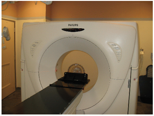Figure 12.11. Photograph of Phillips computed tomography simulator at the University of Minnesota.

Figure 12.12. Photograph of Siemens positron emission tomography/computed tomography at the University of Minnesota.

A PET/CT unit consists of PET and CT scanners combined together with a common patient couch (Fig. 12.12). Because the patient position on the couch is kept constant for both of the scanning procedures, it is relatively straightforward to fuse the information from the two scanners. The composite simulation image contains more information than is possible by a CT simulator alone.

The physics of PET involves positron-electron annihilation into photons. For example, a radiolabeled compound such as fluorodeoxyglucose (FDG) incorporates ¹⁸F as the positron-emitting isotope. FDG is an analog of glucose that accumulates in metabolically active cells. Because tumor cells are generally more active metabolically than the normal cells, an increased uptake of FDG is positively correlated with the presence of tumor cells and their metabolic activity. When the positron is emitted by ¹⁸F, it annihilates a nearby electron, with the emission of two 0.511-MeV photons in opposite directions. These photons are detected by ring detectors placed in a circular gantry surrounding the patient. From the detection of these photons, computer software (e.g., filtered back-projection algorithm) reconstructs the site of the annihilation events and the intervening anatomy. The site of increased FDG accumulation, with the surrounding anatomy, is thereby imaged with a resolution of approximately 4 mm.

Combining PET with CT scanning has several advantages:

Superior quality CT images with their geometric accuracy in defining anatomy and tissue density differences are combined with PET images to provide physiologic imaging, thereby differentiating malignant tumors from the normal tissue on the basis of their metabolic differences.
PET images may allow differentiation between benign and malignant lesions well enough in some cases to permit tumor staging.
PET scanning may be used to follow changes in tumors that occur over time and with therapy.
By using the same treatment couch for a PET/CT scan, the patient is scanned by both modalities without moving (only the table is moved between scanners). This minimizes positioning errors in the scanned data sets from both units.
By fusing PET and CT scan images, the two modalities become complementary. Although PET provides physiologic information about the tumor, it lacks correlative anatomy and is inherently limited in resolution. CT, on the other hand, lacks physiologic information but provides superior images of anatomy and localization. Therefore, PET/CT provides combined images that are superior to either PET or CT images alone.

12.3. TREATMENT VERIFICATION

A. PORT FILMS

The primary purpose of port filming is to verify the treatment volume under actual conditions of treatment. Although the image quality with the megavoltage x-ray beam is poorer than with the diagnostic or the simulator film, a port film is considered mandatory not only as a good clinical practice, but also as a legal record.

As a treatment record, a port film must be of sufficiently good quality so that the field boundaries can be described anatomically. However, this may not always be possible due to either very high beam energy (10 MV or higher), large source size (cobalt-60), large patient thickness (>20 cm), or poor radiographic technique. In such a case, the availability of a simulator film and/or a treatment diagram with adequate anatomic description of the field is helpful. Anatomic interpretation of a port film is helped by obtaining a full-field exposure on top of the treatment port exposure.

The radiographic technique significantly influences the image quality of a port film. The choice of film and screen as well as the exposure technique is important in this regard. Droege and Bjärngard (12) have analyzed the film screen combinations commonly used for port filming at megavoltage x-ray energies. Their investigation shows that the use of a single emulsion film with the emulsion adjacent to a single lead screen¹ between the film and the patient is preferable to a double emulsion film or a film with more than one screen. Thus, for optimum resolution, one needs a single emulsion film with a front lead screen and no rear screen. Conventional nonmetallic screens are not recommended at megavoltage energies. Although thicker metallic screens produce a better response, an increase in thickness beyond the maximum electron range produces no further changes in resolution (12).

Certain slow-speed films, ready packed but without a screen, can be exposed during the entire treatment duration. A therapy verification film such as Kodak XV-2 is sufficiently slow to allow an exposure of up to 200 cGy without reaching saturation. In addition, such films can be used to construct compensators for both the contour and tissue heterogeneity (13).

B. ELECTRONIC PORTAL IMAGING

Major limitations of port films are (a) viewing is delayed because of the time required for processing, (b) it is impractical to do port films before each treatment, and (c) film image is of poor quality especially for photon energies greater than 6 MV. Electronic portal imaging overcomes the first two problems by making it possible to view the portal images instantaneously (i.e., images can be displayed on computer screen before initiating a treatment or in real time during the treatment). Portal images can also be stored on computer disks for later viewing or archiving.

On-line electronic portal imaging devices (EPIDs) are currently being clinically used in most institutions, and are commercially available with all modern linacs. In the past some of the systems were video based. In such a system, the beam transmitted through the patient excited a metal fluorescent screen, which was viewed by a video camera using a 45-degree mirror (14, 15, 16, 17, 18) (Fig. 12.13). The camera was interfaced to a microcomputer through a frame-grabber board for digitizing the video image. The images were acquired and digitized at the video rate of 30 frames per second. An appropriate number of frames were averaged to produce a final image. Depending on the computer software, the image data could be further manipulated to improve the image quality or perform a special study.

Another class of EPIDs that has been used in the past consists of a matrix of liquid ion chambers used as detectors (19,20). These devices are much more compact than the video-based systems and are comparable in size to a film cassette, albeit a little heavier. One such system developed at The Nederlands Kanker Institute consists of a matrix of 256 × 256 ion chambers
containing an organic fluid and a microcomputer for image processing. Figure 12.14 shows an image obtained with such a device.

Figure 12.13. Schematic diagram of the video-based electronic portal imaging device.

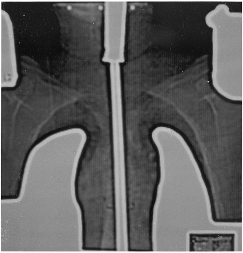Figure 12.14. Example of a portal image. (Courtesy of Varian Associates, Palo Alto, CA.)

Today, most commercial EPIDs use flat panel arrays of solid state detectors based on amorphous silicon (a-Si) technology (Fig. 12.15). Flat panel arrays are compact, making it easier to mount on a retractable arm for positioning in or out of the field. Within this unit a scintillator converts the radiation beam into visible photons. The light is detected by an array of photodiodes implanted on an amorphous silicon panel. Amorphous silicon is used because of its high resistance to radiation damage (21). The photodiodes integrate the light into charge captures. This system offers better image quality than the previous system using liquid ion chambers.

C. CONE-BEAM CT

A conventional CT scanner has a circular ring of detectors, rotating opposite an x-ray tube. However, it is possible to perform CT scans with detectors imbedded in a flat panel instead of a circular ring. CT scanning that uses this type of geometry is known as cone-beam computed tomography (CBCT).

In cone-beam CT, planar projection images are obtained from multiple directions as the source with the opposing detector panel rotates around the patient through 180 degrees or more. These multidirectional images provide sufficient information to reconstruct patient anatomy in three dimensions, including cross-sectional, sagittal, and coronal planes. A filtered back-projection algorithm is used to reconstruct the volumetric images (22).

CBCT systems are commercially available as accessories to linear accelerators. They are mounted on the accelerator gantry and can be used to acquire volumetric image data under
actual treatment conditions, thus enabling localization of planned target volume and critical structures before each treatment. The system can be implemented either by using a kilovoltage x-ray source or the megavoltage therapeutic source.

Figure 12.15. Varian Portalvision system with a panel of amorphous silicon detectors mounted on the accelerator gantry. The mounting arm swings into position for imaging and out of the way when not needed. (Courtesy of Varian Associates, Palo Alto, CA.)

C.1. Kilovoltage CBCT

Kilovoltage x-rays for a kilovoltage CBCT (kVCBCT) system are generated by a conventional x-ray tube that is mounted on a retractable arm at 90 degrees to the therapy beam direction. A flat panel of x-ray detectors is mounted opposite the x-ray tube. The imaging system thus provided is quite versatile and is capable of cone-beam CT as well 2-D radiography and fluoroscopy. Figure 12.16 shows a picture of Elekta Synergy. Figure 12.17 is an example of kVCBCT of a lung cancer patient. It should be mentioned that the accelerator-mounted imaging systems are under constant development and some advertised features may be works in progress or currently not approved by the Food and Drug Administration. The reader can get the updated information by contacting the manufacturers or visiting their web sites.

The advantages of a kVCBCT system are its ability to (a) produce volumetric CT images with good contrast and submillimeter spatial resolution, (b) acquire images in therapy room coordinates, and (c) use 2-D radiographic and fluoroscopic modes to verify portal accuracy, management of patient motion, and making positional and dosimetric adjustments before and during treatment. The use of such systems will be further discussed in Chapter 25 on image-guided radiation therapy (IGRT).

C.2. Megavoltage CBCT

Megavoltage cone-beam CT (MVCBCT) uses the megavoltage x-ray beam of the linear accelerator and its EPID mounted opposite the source. EPIDs with the a-Si flat panel detectors are sensitive enough to allow rapid acquisition of multiple, low-dose images as the gantry is rotated through 180 degrees or more. From these multidirectional 2-D images, volumetric CT images are reconstructed (23, 24, 25).

Figure 12.16. Elekta Synergy linear accelerator with on-board imaging equipment. (Courtesy of Dr. Kiyoshi Yoda, Elekta K.K., Kobe, Japan.)

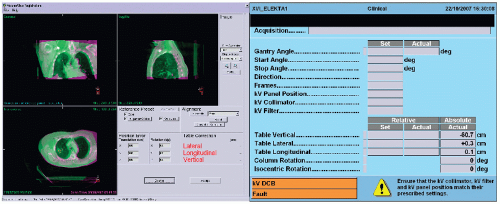Figure 12.17. Example of kilovoltage cone-beam computed tomography images of a lung cancer patient.

The MVCBCT system has a reasonably good image quality for the bony anatomy and, in some cases, even for soft tissue targets. MVCBCT is a great tool for on-line or pretreatment verification of patient positioning, anatomic matching of planning CT and pretreatment CT, avoidance of critical structures such as spinal cord, and identification of implanted metal markers if used for patient setup.

Although kVCBCT has better image quality (resolution and contrast), MVCBCT has the following potential advantages over kVCBCT:

Less susceptibility to artifacts due to high-Z objects such as metallic markers in the target, metallic hip implants, and dental fillings
No need for extrapolating attenuation coefficients from kV to megavoltage photon energies for dosimetric corrections

¹Such a sheet of lead acts as an intensifying screen by means of electrons ejected from the screen by photon interactions. These electrons provide an image on the film that reflects the variation of beam intensity transmitted through the patient.

12.4. CORRECTIONS FOR CONTOUR IRREGULARITIES

As mentioned at the beginning of this chapter, basic dose distribution data are obtained under standard conditions, which include homogeneous unit density phantom, perpendicular beam incidence, and flat surface. During treatment, however, the beam may be obliquely incident with respect to the surface and, in addition, the surface may be curved or irregular in shape. Under such conditions, the standard dose distributions cannot be applied without proper modifications or corrections.

Before the advent of treatment planning computers, isodose charts were corrected for contour irregularity by manual methods. These methods have given way to more accurate analytical methods that are incorporated into the computer treatment planning software. Accuracy and versatility of contour corrections made by a treatment planning system depend on the dose calculation algorithm used (e.g., a semiempirical correction-based algorithm or a model-based algorithm simulating radiation transport). In either case, the point of calculation is assigned its actual depth along the ray line emanating from the radiation source position.

Although manual methods are no longer used for routine treatment planning, these methods are discussed below because they illustrate the basic principles of contour correction and may be used as a rough check of computer corrections. The following three methods may be used for angles of incidence of up to 45 degrees for megavoltage beams and of up to 30 degrees from the surface normal for orthovoltage x-rays (26).

A. EFFECTIVE SOURCE TO SURFACE DISTANCE METHOD

Consider Figure 12.18 in which the source to surface distance (SSD) varies across the field with the beam incident on an irregularly shaped patient contour. It is desired to calculate the percent depth dose at point A (i.e., dose at A as a percentage of D_max dose at point Q). The diagram shows that the tissue deficit above point A is h cm and the reference depth of D_max is d_m. If we note that the percent depth dose does not change rapidly with SSD (provided that the SSD is large), the relative depth dose distribution along the line joining the source with point A is unchanged when the isodose chart is moved down by the distance h and positioned with its surface line at S′ S′. Suppose D_A is the dose at point A. Assuming beam to be incident on a flat surface located at S′ – S′,

Figure 12.18. Diagram illustrating methods of correcting dose distribution under an irregular surface such as S–S. The solid isodose curves are from an isodose chart that assumes a flat surface located at S′-S′. The dashed isodose curves assume a flat surface at S″-S″ without any air gap.

where P′ is percent depth dose at A relative to D′_max at point Q′. Suppose P_corr is the correct percent depth dose at A relative to D_max at point Q. Then,