Ultrasound
14.0 INTRODUCTION
The characteristics, properties, and production of ultrasound for clinical applications are described. Ultrasound interaction with tissues, instrumentation, equipment, image acquisition, processing, and display demonstrate how useful acoustic properties can be obtained, including tissue stiffness and blood velocity determinations. Common artifacts, bioeffects, and safety aspects are also considered.
14.1 CHARACTERISTICS OF SOUND
Sound is mechanical energy that propagates through a continuous medium by the compression (high pressure) and rarefaction (low pressure) of particles that comprise it. For ultrasound, the mechanical force is a transducer, composed of an expanding and contracting group of crystal elements creating local periodic compressions and rarefactions in the tissue medium. Mechanical energy travels at the speed of sound into the patient and “particles” of the tissue transfer energy much like a compressible spring, traveling as a longitudinal wave (Fig. 14-1).
1. Wavelength, Frequency, Speed
a. Wavelength (λ): distance between two repeating points in a periodic wave (i.e., a cycle), (e.g., mm).
b. Frequency (f) is the cycle repetition per second (s), in Hertz (Hz), where 1 Hz = 1 cycle/s.
(i) Less than 15 Hz is infrasound; 15 to 20 kHz is audible sound; greater than 20 kHz is ultrasound Medical ultrasound: 1 to 20 MHz, up to 50 MHz and beyond for specialized applications
c. Period: time duration of one wave (cycle) and is equal to 1/f
d. Speed of sound, c: distance traveled per unit time is equal to the product of wavelength and frequency

(i) Speed of sound units: m/s (meters/second), cm/s, mm/µs.
(ii) c varies in a medium, based on compressibility, stiffness, and density characteristics; tissues with high compressibility = slow speed (e.g., air); greater stiffness = high speed (e.g., bone) (Table 14-1).
e. Using c = 1.54 mm/µs, the wavelength in mm of soft tissue = 1.54 mm/f (MHz), thus the wavelength of a 10-MHz beam is easily calculated, as 1.54/10 = 0.154 mm and for a 2-MHz beam as 1.54/2 = 0.77 mm (Fig. 14-2).
f. Higher frequencies provide better resolution, but higher attenuation and limited depth penetration.
2. Pressure and Intensity
a. Pressure (P), expressed as Newton per square meter (N/m2) with SI unit of pascal (Pa); “pressure amplitude” refers to the magnitude of change in pressure: note—earth’s atmospheric pressure = 100,000 Pa and ultrasound imaging peak pressure is 1,000,000 Pa or 1 MPa—the peak US intensity is about 10 times higher than earth atmospheric pressure.
b. Intensity, I, is a measure of average power per unit area and is proportional to the square of the pressure amplitude, I ∝ P2; medical diagnostic ultrasound intensity levels are milliwatts/cm2.
c. Relative pressure and intensity levels are scaled using the decibel (dB), a unitless value.


▪ FIGURE 14-1 Top: Ultrasound energy is generated by a mechanical displacement of a elastic medium, modeled as a compressible spring. An inward and outward force of a piston coupled to the medium creates increased pressure (compression) and decreased pressure (rarefaction) in a cyclical manner. Mid: Side view of transducer with crystal elements that expand and contract at a high frequency shows energy propagation as a wave with the wavelength equal to the distance of one cycle. Bottom: Ultrasound propagates in the medium as a longitudinal wave. F. 14-2

▪ FIGURE 14-2 Ultrasound wavelength is determined by the frequency and the speed of sound in the propagation medium. Wavelengths in soft tissue are calculated for 2-, 5-, and 10-MHz ultrasound sources for soft tissue (blue). A comparison of wavelength in fat (red) to soft tissue at 5 MHz is also shown. F. 14-3
TABLE 14-1 DENSITY, SPEED OF SOUND, AND ACOUSTIC IMPEDANCE FOR TISSUES AND MATERIALS RELEVANT TO MEDICAL ULTRASOUND
MATERIAL
DENSITY (kg/m3)
C (m/s)
Z (rayls)a
Air
1.2
330
3.96 × 10²
Lung
300
600
1.80 × 10³
Fat
924
1,450
1.34 × 10⁶
Water
1,000
1,480
1.48 × 10⁶
“Soft Tissue”
1,050
1,540
1.62 × 10⁶
Kidney
1,041
1,565
1.63 × 10⁶
Blood
1,058
1,560
1.65 × 10⁶
Liver
1,061
1,555
1.65 × 10⁶
Muscle
1,068
1,600
1.71 × 10⁶
Skull bone
1,912
4,080
7.8 × 10⁶
PZT
7,500
4,000
3.0 × 10⁷
a Acoustic impedance is the product of density and speed of sound. The named unit, rayl, has base units of kg/(m2s) for values listed in the column. Acoustic impedance directly relates to the propagation characteristics of ultrasound in each medium and is the basis for echo formation.
(i) Pressure is proportional to voltage, so Equation 14-2 compares induced voltages of echoes.
(ii) Pressure or voltage comparisons have a factor of 2× higher values on dB scale relative to intensity.
(iii) Intensity ratio of 106 (e.g., incident pulse intensity is 106 greater than echo intensity) = 60 dB (Eq. 14-3).
(iv) Change of 10 in the relative intensity dB scale = order of magnitude (10 times) change.
(v) Change of 20 is equal to two orders of magnitude (100 times) change, and so forth.
(vi) Intensity ratio greater than 1, dB scale is positive; less than 1, dB scale is negative.
(vii) Loss of 3 dB (-3 dB) represents a 50% loss of signal intensity, the “half-value” thickness (HVT).
e. Ultrasound energy imparted to the medium depends on the pressure amplitude variations generated by the degree of transducer expansion and contraction through transmit gain.
TABLE 14-2 INTENSITY RATIO AND CORRESPONDING DECIBEL VALUES | |||||||||||||||||||||||||||||||||||
|---|---|---|---|---|---|---|---|---|---|---|---|---|---|---|---|---|---|---|---|---|---|---|---|---|---|---|---|---|---|---|---|---|---|---|---|
|
14.2 INTERACTIONS OF ULTRASOUND WITH TISSUES
Interactions of ultrasound are chiefly based on the acoustic impedance of tissues and result in reflection, refraction, scattering, and absorption of the ultrasound energy.
1. Acoustic Impedance, Z: a measure of tissue stiffness and flexibility
a. Equal to the product of density and speed of sound: Z = ρc
(i) ρ is the density in kg/m3; c is the speed of sound in m/s.
b. Sound energy transfer efficiency from one tissue to another is dependent on differences in Z.
(i) For similar Z, a large fraction of incident intensity will be transmitted through a boundary.
(ii) For wide differences in Z, most incident intensity will be reflected at the boundary.
(iii) Most soft tissues have a similar Z, allowing ultrasound to penetrate deep into the body.
2. Reflection back to the transducer
a. A beam traveling perpendicular (normal incidence = 90°) to boundary between two tissues (Fig. 14-3A).
b. The fraction of incident intensity reflected at a boundary is the intensity reflection coefficient, RI:

Subscripts 1 and 2 represent tissues that are proximal and distal to the boundary, respectively.
c. Intensity transmission coefficient TI is equal to 1 – RI.
d. Example of reflection at fat/muscle interface, Zfat = 1.34, Zmuscle = 1.71, 1.5% of intensity is reflected:

e. With air, the reflection coefficient is 1, thus 100% of incident intensity is reflected.
f. For nonnormal incidence, the reflected angle = incident angle relative to the normal direction.
3. Refraction
a. A change in direction of the transmitted ultrasound pulse when the incident pulse is not perpendicular to the tissue boundary, and the speeds of sound in the two tissues are different (Fig. 14-3B).
b. Angle of refraction determined by Snell law: ; approximated as
  .
.

▪ FIGURE 14-3 Reflection and refraction of ultrasound occur at tissue boundaries with differences in acoustic impedance, Z. A. With perpendicular incidence (90°), a fraction of the beam is transmitted, and a fraction of the beam is reflected toward the source at a tissue boundary. B. With nonperpendicular incidence (≠90°), the reflected fraction of the beam is directed away from the transducer at an angle θr = θi and the transmitted fraction of the beam is refracted in the transmission medium at a transmitted angle greater than the incident angle (θt > θi) when c2 > c1, and less than the incident angle when c1 > c2. F. 14-4
4. Scattering
a. Arises from objects and interfaces within tissues with size on the order of ultrasound wavelength.
(i) Low frequencies (1 to 5 MHz) with longer λ, boundaries appear specular (mirror-like)
(ii) High frequencies (greater than 5 to 15 MHz) with shorter λ, boundaries are nonspecular (Fig. 14-4)
b. Tissue signatures arise from different organs due to internal structure and echo correlation patterns.
c. Hypoechoic and hyperechoic are terms describing characteristics of tissues in terms of the relative intensity of the backscattered signal.
5. Absorption and Attenuation
a. Attenuation is the loss of US intensity with distance traveled from scattering and absorption.
b. Expressed in decibels (dB), with an average attenuation of 0.5 dB/(cm-MHz) (See Table 14-4, textbook).
c. Ultrasound attenuation occurs exponentially with depth and more rapidly with frequency (Fig. 14-5).
d. Choice of ultrasound transducer frequency is strongly dependent on required depth of imaging.
e. Example: calculate the relative ratio (incident pulse to returning echo) of a 5 MHz US wave traveling to a depth of 4 cm with a 100% reflective boundary. Answer: 5 MHz × 0.5 dB/(cm-MHz) = 2.5 dB/cm attenuation for a total travel distance of 8 cm (to and from reflector), loss of US intensity is thus 2.5 dB/cm × 8 cm = 20 dB. The relative ratio is thus 20 dB = 10 log (Iincident/Iecho); Iincident = 100 Iecho.
 ▪ FIGURE 14-4 Specular and nonspecular boundary characteristics are dependent on the wavelength of the incident ultrasound pulse, leading to coherent and diffuse returning echo patterns. At higher frequencies, a significant fraction of the echoes do not return.  F. 14-5 F. 14-5 |
 ▪ FIGURE 14-5 Ultrasound attenuation occurs exponentially with depth. The plots are estimates of a single frequency US wave with an attenuation coefficient of 0.5 dB/(cm-MHz). The total distance traveled is twice the penetration depth at the reflection boundary.  F. 14-6 F. 14-6 |
14.3 ULTRASOUND TRANSDUCERS
Ultrasound is transmitted and received by a transducer array, composed of hundreds of small ceramic elements with electromechanical (piezoelectric) properties, connected to controlling electronics and contained in a handheld, plastic housing with other components essential to proper operation.
1. Piezoelectric Materials
a. Lead zirconate titanate (PZT)—synthetic material composed of aligned dipole structure (Fig. 14-6).
b. Electrodes attached to each surface of PZT thickness provide the ability to receive and produce US.
c. Small mechanical displacements by returning waves in the receive mode create voltage differences of microvolts (µV).
d. Externally applied voltage pulse (approximately 100 V) in the transmit mode reorients the PZT into crystal “thickness” contraction or expansion togenerate ultrasound energy.

▪ FIGURE 14-6 The piezoelectric element is composed of aligned molecular dipoles. A. A mechanical displacement (e.g., returning echo) generates small displacement with the increased pressure of the compression wave causing contraction and the decreased pressure of the rarefaction causing expansion, with small changes in surface voltage measured by the electrodes. B. An external voltage source applied to the surface over several microseconds causes compression or expansion from equilibrium in response to electrical attraction or repulsion force on the dipolar internal structure of the PZT. F. 14-7
e. The US pulse is created using a short-duration voltage spike in the compression mode; the PZT vibrates at a natural frequency in the thickness mode of λ/2; crystal thickness determines frequency (Fig. 14-7).
2. Resonance Frequency, Damping, Absorbing, and Matching Layers
a. Transducer arrays are composed of multiple elements, each attached with electrode wires.
b. Excitation of undamped crystals will result in a long-duration, narrow bandwidth frequency (Fig. 14-8A).
(i) “Q” factor represents the purity of produced sound: Q = f0/bandwidth.
(ii) A damping layer is required to shorten pulse width, which increases the bandwidth
(iii) US imaging requires transducers with low Q to obtain a short spatial pulse length.
c. Compression in thickness mode causes expansion in the width and height of the elements (Fig. 14-8B).

▪ FIGURE 14-7 A short duration voltage spike causes the piezoelectric element to vibrate at its natural frequency, f0, equal to λ/2, determined by the thickness. A thinner crystal operates at a higher frequency. F. 14-8.

▪ FIGURE 14-8 A. The single element crystal showing thickness, height, and width dimensions. B. A section of a multielement array at equilibrium, expansion, and contraction modes, illustrating variation in the height and width. This can cause emission of off-axis ultrasound energy and generate artifacts. F. 14-9
d. US is emitted in both directions upon PZT excitation, requiring the use of an adjacent absorption layer.
e. A matching layer provides the interface between the PZT and tissue to maximize transmission.
(i) Matching layer thickness is equal to ¼ λ with a speed of sound between PZT and soft tissue.
(ii) Acoustic coupling gel is also used to improve contact and eliminate air pockets.
f. The composite structure of the transducer element array and housing are shown in Figure 14-9.
3. Broad Bandwidth “Multifrequency” Transducer Operation
a. Transducer elements are manufactured with many small PZT rods backfilled with epoxy.
b. Properties of these elements provide a better acoustic impedance match with tissue and can be operated over a selectable range of frequencies due to the composite characteristics of the material.
c. Excitation pulses of specific square wave voltage pulses of 1 to 3 cycles selects the center frequency across the available bandwidths of the transducer array.
d. Broad bandwidth response of the transducer array (Fig. 14-10) permits reception of echoes at specific frequencies, useful for native tissue harmonic imaging (see Section 14.6.5).

▪ FIGURE 14-9 A. The transducer is composed of a housing, electrical insulation, and a composite of active element layers, including the PZT crystal, damping block and absorbing material on the backside, and a matching layer on the front side of the multielement array. B. The ultrasound spatial pulse length is based upon the damping material causing a ring-down of the element vibration. For imaging, a pulse of 2 to 3 cycles is typical, with a wide frequency bandwidth, while for Doppler transducer elements, less damping provides a narrow frequency bandwidth. F. 14-10

▪ FIGURE 14-10 Multifrequency transducer transmit and receive response to operational frequency bandwidths, allows the operator to select an appropriate transmit and receive frequency depending on the type of exam, type of transducer, the transducer bandwidth range, and the need for penetration depth (selecting lower frequency) or spatial resolution (selecting higher frequency). The transducer response shown has a selectable frequency range of 4 to 10 MHz. F. 14-11
4. Transducer Arrays
a. Linear, curvilinear, and phased array operation are most common for diagnostic ultrasound (Fig. 14-11).
b. Linear and curvilinear arrays activate a subset of elements producing a single transmit beam pulse.
(i) Subsequent receive mode is activated to listen to echoes from depth
(ii) Activation of a different subset of adjacent elements produces another beam pulse.
(iii) This continues for all of the elements across the array, which is then repeated.
c. Phased transducer arrays activate all elements in the array, and with fine and ultrafine transmit delay timing, electronic steering of the beam can be achieved, producing a sector-scan format.
d. Intracavitary transducer arrays use both linear and phased array operation for imaging.
e. Mechanical/electronic array scanners are used for real-time 3D imaging (e.g., fetal imaging, see text for details).
 ▪ FIGURE 14-11 A. The linear array transducer activates a subgroup of transducer elements to produce an ultrasound beam directed perpendicular to the array, repeating with incremental shifting of the subgroup element by element. A rectangular field of view is produced. B. The curvilinear (also known as convex) array operates with subgroup transducer element excitation, like the linear array. A convex arrangement produces a trapezoidal field of view, with good coverage proximally and extended coverage distally. C. A phased array transducer produces a beam from the near-simultaneous excitation of all array elements. The beam can be electronically steered across the FOV using transmit delay excitation patterns. A sector scan format is produced with incremental time delay patterns to control the direction and number of lines across the FOV.  F. 14-12A, F. 14-13A, F. 14-14B F. 14-12A, F. 14-13A, F. 14-14B |
14.4 ULTRASOUND BEAM PROPERTIES
The transducer-generated US beam propagates as a longitudinal wave from the transducer surface into the propagation medium and exhibits two distinct beam patterns: a slightly converging beam out to a distance determined by the geometry and frequency of the transducer (the near field) and a diverging beam beyond that point (the far field). Other considerations include US beam focusing, the generation of side lobes and grating lobes, and the spatial resolution determinants in a US beam, including axial, lateral, and elevational.
1. The Near Field
a. Also known as the Fresnel zone, is adjacent to the transducer face out to the minimum beam diameter.
(i) A converging beam profile is due to interference patterns from the multiple US sources.
(ii) “Huygens principle” describes the transducer as an infinite number of point sources.
b. The near field depth increases with excitation radius, r, and inverse to US wavelength, λ: length = r2/λ.
(i) Lateral beam dimension for subarray of linear transducer is about ½ size of excitation footprint.
c. Pressure amplitude changes are complex in the near field and vary rapidly (Fig. 14-12).

▪ FIGURE 14-12 A linear array transducer subgroup excitation (top) and the expanded beam profile (middle) shows the near-field and far-field characteristics of the ultrasound beam. The near field is characterized as a collimated beam, and the far-field begins when the beam diverges. Point emitters (left middle) generate constructive and destructive interference patterns that cause beam collimation and large pressure amplitude variations in the near field (lower diagram). Beam divergence occurs in the far-field, where pressure amplitude monotonically decreases with propagation distance. F. 14-16
2. The Far Field
a. Also known as the Fraunhofer zone, begins at end of the near field
(i) Characterized by diverging wave and monotonically decreasing pressure (Fig. 14-12)
3. Transducer array beam focusing
a. Transmit focus is achieved by applying timing delays between transducer elements.
(i) This occurs within the subgroup of elements for linear and curvilinear arrays and for all elements for phased array transducers (Fig. 14-13).
(ii) Focal zones can occur at various depths depending on the delays between element excitations.
b. Receive focus is dynamically applied to all active elements during the reception of the echoes.
(i) Proximal echoes returning from a boundary interface are more concave—timing delays from central elements are longer relative to the peripheral elements to achieve phase coherence (Fig. 14-13).
(ii) Distal echoes have a less concave echo pattern, and the variable timing circuitry adjusts accordingly.

▪ FIGURE 14-13 Transmit and Receive focusing. A. Transmit focusing is achieved by implementing a programmable delay time (beamformer electronics) for the excitation of the individual transducer elements in a concave pattern with outer elements energized first. The individual ultrasound pulses converge to a minimum beam diameter (the focal distance) at a predictable depth in tissue. B. Dynamic receive focusing uses receive beamformer electronics to dynamically adjust delay times for processing the received echo signals. This compensates for differences in arrival time across the array as a function of time (depth of the echo) and results in phase alignment of the echo signals by all elements to achieve a good signal output as a function of time. F. 14-17
4. Side Lobes and Grating Lobes
a. Side lobes represent US intensity created from the element width and height expansion and contraction.
(i) Energy is directed adjacent to the main beam area in the forward direction (Fig. 14-14A).
(ii) Side lobes can easily generate echoes that map into the main beam (see section on artifacts).
b. Grating lobes result from the discrete excitations in multielement arrays.
(i) US intensity is emitted at wide angles (Fig. 14-14B).
(ii) The intensity of grating lobes is substantially less than side lobes.
c. For both side lobes and grating lobes, intensity is diminished with low Q operation (see Section 14.3.2).

▪ FIGURE 14-14 Side lobes and grating lobes. A. Side lobes represent ultrasound energy produced outside of the main ultrasound beam along the same beam direction caused by height and width variations of the transducer elements. B. Grating lobes represent the emission of energy at large angles relative to the direction of the beam caused by the discrete nature of the multielement transducer array. At the edges of the array, energy is emitted that does not undergo interference as shown by the inset diagram. The grating lobe intensity is low relative to the intensity of the main beam or side lobes. F. 14-18
5. Spatial Resolution
US resolution has three separate components: Axial, Lateral, and Elevational (Slice Thickness) (Fig. 14-15). Visibility of detail in the image is determined by the volume and dimensions of the acoustic pulse.

▪ FIGURE 14-15 A. The axial, lateral, and elevational (slice-thickness) contributions in three dimensions are shown for a phased-array transducer ultrasound beam. Axial resolution, along the direction of the beam, is independent of depth; lateral resolution and elevational resolution are strongly depth-dependent. Lateral resolution is determined by transmit and receive focus electronics; elevational resolution is determined by the height of the transducer elements. At the focal distance, axial is better than lateral, and lateral is better than elevational resolution. B. Elevational resolution profile with an acoustic lens across the transducer array produces a weak focal zone in the slice thickness direction. F. 14-19
a. Axial resolution is also known as linear, range, longitudinal, or depth resolution.
(i) The ability to distinguish closely spaced objects in the direction of the US beam.
(ii) Is equal to ½ spatial pulse length (SPL), where SPL = product of wavelength and #cycles per pulse.
(iii) Short SPL is achieved with higher damping of transducer elements, typically 2 to 3 cycles, and higher frequency of operation (shorter wavelength) (Fig. 14-16).
b. Lateral resolution is also known as azimuthal resolution.
(i) The ability to distinguish closely spaced objects perpendicular to the direction of the US beam, and in the plane of the image.
(ii) Beamwidth is the determining factor, which changes as a function of depth (Fig. 14-17).
(iii) Lateral focal zones can be established to create a narrower beam diameter at a specified depth.
(iv) Multiple focal zones can provide good resolution over a range of depths (Fig. 14-18).
(v) Drawbacks of focal zone placement are a loss of temporal resolution and possible transition band artifacts (see section on Ultrasound Artifacts).

▪ FIGURE 14-16 Axial resolution is equal to ½ SPL. Tissue boundaries that are separated by a distance greater than ½ SPL produce echoes from the first boundary that are completely distinct from echoes reflected from the second boundary, whereas boundaries with less than ½ SPL result in overlap of the returning echoes. Higher frequencies reduce the SPL and thus improve the axial resolution, as shown in the lower diagram. F. 14-20

▪ FIGURE 14-17 Lateral resolution is a measure of the ability to discern objects perpendicular to the direction of beam travel and is determined by the beam diameter. Point targets in the beam are averaged over the effective beam diameter in the ultrasound image as a function of depth. Best lateral resolution occurs at the focal distance; good resolution occurs over the focal zone. F. 14-21
c. Elevational resolution is also known as slice thickness resolution.
(i) Like lateral resolution, elevational is depth dependent with a focal zone (Fig. 14-19).
(ii) “1.5D” arrays can provide multiple elevational focal zones.
 ▪ FIGURE 14-18 Linear and phased array transducers have multiple user-selectable transmit and receive focal zones implemented by the beamformer electronics. For this phased array transducer, each focal zone requires the transmit beamformer excitation of the active array for a given focal distance. Subsequent processing meshes the independently acquired data to enhance the lateral focal zone over a greater distance, at the expense of reduced frame rate.  F. 14-22 F. 14-22 |
 ▪ FIGURE 14-19 Elevational resolution with multiple transmit focusing zones is achieved with “1.5D” transducer arrays to reduce the slice thickness profile over an extended depth. Five to seven rows of discrete arrays replace the single array. Phase delay timing provides focusing in the elevational plane, like that used for lateral transmit and receive focusing.  F. 14-23 F. 14-23 |
14.5 IMAGE DATA ACQUISITION AND PROCESSING
Images are acquired using a pulse-echo mode of ultrasound production and detection. Each pulse is directionally transmitted into the patient. Partial reflections from tissue boundaries at normal incidence create echoes that return to the transducer as a function of travel time and depth, along a corresponding line in the ultrasound image. The receiver detects the echoes, and the process is repeated incrementally across the field of view to sequentially construct the image line by line. Data acquisition and image formation using the pulse-echo approach requires several hardware components: the beamformer, pulser, receiver, amplifier, scan converter/image memory, and display system (Fig. 14-20).
1. Beamformer: generates electronic delays for transmit/receive focusing and beam steering
a. Computer logic controls pulser, transmit/receive switch, preamps, analog to digital amplifiers
2. Pulser (Transmitter)
a. Provides voltage for exiting transducer elements; controls output transmit power

▪ FIGURE 14-20 Components of the ultrasound imager. This schematic depicts the design of a digital acquisition/digital beamformer system, where each of the transducer elements in the array has a pulser, transmit-receive switch, preamplifier, swept gain, and analog to digital converter (ADC). Swept gain reduces the dynamic range of the signals prior to digitization. The beam former provides focusing, steering, and summation of the beam; the receiver processes the data for optimal signal to noise ratio, and the scan converter produces the output image rendered on the monitor. F. 14-24A
3. Transmit/Receive Switch
a. Isolates high-voltage associated with excitation (150 V) to voltage associated with echoes (approximately µV)
b. “Ring-down” time—the time required for the transducer array to switch from excitation to reception
4. Pulse-Echo Operation
a. Ultrasound intermittently transmits over a short period (approximately 1 µs) and then receives echoes (approximately 1,000 µs).
b. Depth (D) of a received echo is determined by US speed and distance traveled = 2 × depth. Pertinent equations: (uses units of µs, cm, and speed of sound in cm/µs).
Time to receive echo after pulse: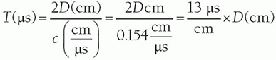
Round trip distance traveled: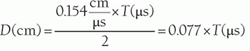
c. Number of pulses/s: pulse repetition frequency (PRF)
d. Time between pulses: pulse repetition period (PRP) (Fig. 14-21)
e. Pulse duration: ratio of the #cycles/pulse to the transducer frequency = “on” time—1 to 2 µs
f. Duty cycle: fraction of “on” time = pulse duration/PRP = approximately 0.2% to 0.4%

▪ FIGURE 14-21 In this example, the pulse-echo timing of data acquisition depicts the initial pulse occurring in a very short time span, the pulse duration, of 1 to 2 µs, and the time between pulses, the pulse repetition period (PRP), of 500 µs. The number of pulses per second, the pulse repetition frequency (PRF), is 2,000/s, or 2 kHz. The indicated depth is ½ of the total travel distance of the pulse/echo for the indicated time. F. 14-25
5. Preamplification and Analog-to-Digital Conversion
a. Returning signals are preamplified prior to analog to digital conversion during swept gain step.
b. Range of voltage amplitude changes can be as much as 120 dB (a factor of 106 for pressure amplitude).

▪ FIGURE 14-22 A phased array transducer (also applicable to linear array operation) produces a pulsed beam that is focused at a programmable depth and receives echoes during the PRP. This figure shows a digital beam former system, with front-end digital electronics (swept gain and ADC) converting the signals prior to beamformer receive focusing. Electronic delays are adjusted as a function of receive time and position to align the phase of the echoes received by each transducer element. The output is summed to form the ultrasound echo train along a specific beam direction. F. 14-26
6. Beam Steering, Dynamic Focusing, and Signal Summation (Fig. 14-22)
a. It is essential to orchestrate the acquisition to achieve a high SNR echo train during the PRP.
b. A combination of preamplification and dynamic focusing produces a stream of reliable acoustic data.
7. Receiver accepts data from the beamformer during the PRP, with subsequent signal processing (Fig. 14-23): preamplification, time gain compensation, logarithmic compression, demodulation, and noise rejection
a. Time gain compensation (Fig. 14-24) is a user-adjustable amplification of returning echoes versus time
(i) Ideal TGC curve makes all equally reflective boundaries at various depths have the same amplitude.
(ii) User adjustment is typical with multiple slider potentiometers or electronic calipers.
b. Dynamic range/logarithmic compression reduces the echo amplitude range for the video display.
c. Demodulation and envelope detection converts the detected signals into a positive, smooth pulse.
d. Noise rejection sets the lower threshold signal level allowed to pass the scan converter.

▪ FIGURE 14-23 A snapshot of data streaming from the beamformer is described. Left column is the processing step, middle is the illustration of the signal, and right is the described output. The user can adjust the time gain compensation (TGC) levels and the noise rejection level. F. 14-27

▪ FIGURE 14-24 A TGC amplifies the acquired signals with respect to time after the initial pulse by operator adjustments. A. Equally reflective boundaries are expected to produce equal echo amplitudes. B. On the operator console, the sonographer interactively adjusts TGC with a set of electronic calipers or slide potentiometers to optimize the gain. F. 14-28
e. Processed signals are passed to the scan converter for gray scale image display.
8. Echo Signal Modes
a. A-mode (amplitude) is the processed signal versus time as shown in Figure 14-23(5), where 1 A-line of data is produced per pulse for conventional line-by-line acquisition.
b. B-mode (brightness) is the conversion of the A-mode amplitude into a B-mode gray scale values.
c. M-mode (motion) is a technique using B-mode signals, a stationary beam, and deflecting the B-mode data as a function of time to evaluate anatomic motion; also known as T-M mode.
9. Scan Converter
a. Generates 2D ultrasound images from B-mode data based on trajectory and time (depth), see Figure 14-20.
b. Data interpolation is used to fill in empty or partially filled pixels in the matrix.
14.6 IMAGE ACQUISITION
The 2D ultrasound image is acquired by sweeping a pulsed ultrasound beam sequentially in a plane over the volume of interest to produce “video clips.” The matrix size and frame rate are dependent on several factors including ultrasound frequency, pulse repetition frequency, the field of view, depth of penetration, number of lines per frame, and line density. Improvements in image acquisition rate are achievable with advanced techniques such as multiline acquisition (MLA), multiline transmission (MLT), plane, and diverging wave imaging. These advances provide frame rates that go well beyond conventional line-by-line acquisitions and create high temporal resolution imaging of several hundred to thousands of frames per second.
1. Real-Time Imaging: frame rate, FOV, depth, sampling tradeoffs (Fig. 14-25)Related posts:

Stay updated, free articles. Join our Telegram channel

Full access? Get Clinical Tree