VI
V2/V3
I. LOG
IPS
S.LOG
DLPFC
AC
RHC
Set 1.A
80 ms
90 ms
100 ms
30 nAm
30 nAm
30 nAm
1.B
80 ms
90 ms
100 ms
50 nAm
50 nAm
50 nAm
Set 2
90 ms
90 ms
100 ms
15 nAm
30 nAm
30 nAm
Set 3.A
80 ms
90 ms
100 ms
30 nAm
30 nAm
30 nAm
3.B
80 ms
90 ms
100 ms
50 nAm
50 nAm
50 nAm
Set 4
90 ms
90 ms
100 ms
100 ms
300 ms*
400 ms*
15 nAm
30 nAm
20 nAm
30 nAm
20 nAm
30 nAm
Set 5
90 ms
90 ms
100 ms
100 ms
300 ms*
400 ms*
80 ms
15 nAm
30 nAm
20 nAm
30 nAm
20 nAm
30 nAm
51 nAm
In the simulated example shown in Fig. 1, a Freesurfer-segmented gray matter/white matter boundary for the simulations was imported into MRIVIEW (Fig. 1a), although the segmentation may also be accomplished within MRIVIEW. The simulated activation timecourses (signal) are shown Fig. 1b. In each case, 100 single trials of real spontaneous background activity were averaged together as the noise trial for each of the 5 participants and for each of the MEG systems (Fig. 1c). Then the signal was embedded within the averaged noise file (Fig. 1d). For all simulated datasets on the web portal, a spherical head model was used for the simulations and modeled data; however, a boundary element model (BEM) is also available in MRIVIEW.
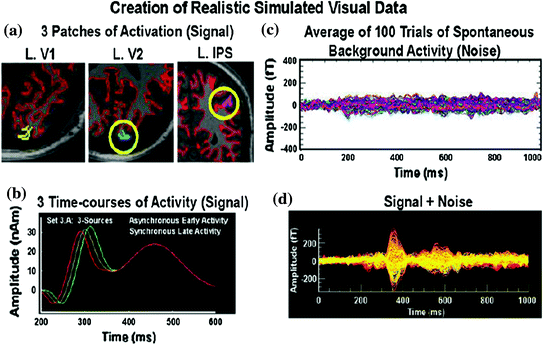

Fig. 1
A Freesurfer-segmented gray matter/white matter boundary for the simulations (shown in red) was imported into MRIVIEW from which patches (a) of simulated activity (b) were generated. 100 passes of spontaneous activity or noise (c) were identified using CTF software (Data Editor) and averaged together using MEGAN. The simulated activity was embedded within the averaged noise file (d) and saved in netCDF format (i.e., a netMEG file in MEGAN). Reprinted from Aine et al. (2012) with permission from Springer
Table 2 shows actual source locations, CSST estimated source locations, and errors when either noise was absent (no-noise) or empirical noise was present for visual simulated data Set 4. CTF head-centered coordinate system is used, where -x points out the back of the head, +y points out the left ear, and +z points out the top of the head. Average error across the 6 sources was 0.1 mm for the no-noise condition and 6.8 mm for the real noise condition. Standard deviation (SDev) is shown for estimated solutions for real-noise simulated data. This table demonstrates that the presence of real noise significantly affects source localization accuracy; however, our CSST solution for the real noise condition was still good for this complicated dataset, and inconsistent with previous critiques of dipole-modeling approaches that state dipole methods cannot accurately localize more than a few point sources of activity. Further, Table 3 lists CSST output when varying the model order (i.e. number of fitted dipoles) for a 3-dipole simulated dataset. The solutions (1–4 Dipoles) shown are for real spontaneous noise. Timecourses (shown as absolute values, bottom) are from the 4-dipole fit to 3-source data. In Table 3 the entries P1, P2, and P3 correspond to the Pk 1, Pk 2, Pk 3 timecourses. Notice that the noise timecourse is low-amplitude and without structure. As this table shows, under-modeling (1- and 2-dipoles) results in large localization errors. In contrast, localization errors are often reduced when over-modeling by 1 dipole (i.e., 4-dipoles for this 3-source dataset). Fortunately, noise sources are often easy to identify by a lack of timecourse structure and low amplitude (lower right panel).
Table 2
Actual and CSST estimated (“no-noise” and “real-noise”) locations for a 6-source, realistic simulation
SET 4 6 sources | Source V3 | Error (mm) | Source I. LOG | Error (mm) | Source IPS | Error (nm) | ||||||
|---|---|---|---|---|---|---|---|---|---|---|---|---|
X | Y | Z | X | Y | Z | X | Y | Z | ||||
Actual | −70.0 | 5.9 | 75.8 | −59.7 | 33.2 | 42.9 | −22.1 | 38.3 | 82.6 | |||
No noise | −69.7 | 6.0 | 75.9 | 0.3 | −59.8 | 33.3 | 42.9 | 0.1 | −22.1 | 38.2 | 82.7 | 0.1 |
Real noise | −61.3 | 4.3 | 74.1 | 9.0 | −55.6 | 31.7 | 44.5 | 4.6 | −18.7 | 28.7 | 71.8 | 14.8 |
SDev (Real) | 0.3 | 2.3 | 1.6 | 1.6 | 0.3 | 0.4 | 1.5 | 1.7 | 0.9 | |||
Source R. frontal | Source AC | Source S. LOG | ||||||||||
|---|---|---|---|---|---|---|---|---|---|---|---|---|
X | Y | Z | X | Y | Z | X | Y | Z | ||||
Actual | 58.1 | −41.5 | 46.2 | 74.1 | −7.0 | 47.8 | −31.3 | −40.7 | 60.3 | |||
No noise | 58.1 | −41.7 | 46.2 | 0.1 | 74.0 | −7.1 | 47.6 | 0.2 | −31.4 | −40.8 | 60.3 | 0.1 |
Real noise | 58.5 | −43.2 | 44.0 | 2.8 | 72.6 | −9.9 | 46.7 | 3.4 | −27.5 | −36.1 | 59.1 | 6.1 |
SDev (Real) | 0.1 | 0.1 | 0.4 | 0.5 | 0.3 | 0.2 | 0.5 | 0.6 | 0.6 | |||
Table 3
Sample output from an automated routine for determining best-fits to 3-source simulated data
Source location | Loc error mm (STD) | Peak amplitude error nAm | Peak latency error ms | Avg Loc error mm | |||||
|---|---|---|---|---|---|---|---|---|---|
Pk 1 | Pk 2 | Pk 3 | Pk 1 | Pk 2 | Pk 3 | ||||
Real spontaneous noise | 1 Dip-V3 | 17.5 (0.15) | 12.4 | 42.5 | 19.6 | 3.0 | 1.0 | 18.0 | 17.5 |
2 Dip-Vl | 9.25 (0.11) | 1.6 | 4.7 | 1.0 | 4.0 | 2.0 | 2.0 | ||
2 Dip-IPS | 7.22 (0.08) | 5.1 | 21.5 | 11.0 | 7.0 | 4.0 | 18.0 | 8.23 | |
3 Dip-V1 | 4.93 (0.13) | 1.1 | 0.45 | 2.2 | 5.0 | 2.0 | 1.0 | ||
3 Dip-V3 | 4.98 (0.12) | 1.9 | 7.1 | 4.1 | 13.0 | 0.0 | 25.0 | ||
3 Dip-IPS | 2.32 (0.05) | 1.3 | 4.6 | 2.8 | 6.0 | 2.0 | 15.0 | 4.08 | |
4 Dip-V1 | 3.11 (0.14) | 0.03 | 3.6 | 0.80 | 4.0 | 2.0 | 6.0 | ||
4 Dip-V3 | 3.51 (0.14) | 3.2 | 5.1 | 2.5 | 1.0 | 1.0 | 29.0 | ||
4 Dip-IPS | 1.56 (0.05) | 1.4 | 5.6 | 3.6 | 5.0 | 2.0 | 18.0 | 2.73 | |
4-Dip-N | Noise | – | – | – | – | – | – | ||
 | |||||||||
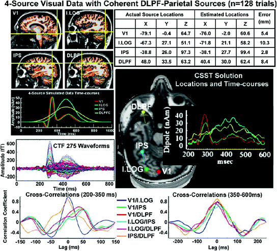
Set 6 (remaining sets are not shown in Table 1) includes late activity (e.g., 400–600 ms) that was synchronous across four cortical sites (V1, I. LOG, IPS, and DLPFC), as is seen in working memory studies (Aine et al. 2006). The upper left panel of Fig. 2 displays the locations of the cortical patches (cortical patches are located at the cross-hairs) while the timecourses assigned to the cortical patches are shown beneath the MRIs. The averaged waveforms (128 trials with signals embedded in real spontaneous noise) seen across the 275 channels of the CTF MEG system are shown in the middle left column. CSST source locations are shown in the upper right panel (see tabled values). The table shows the coordinates of the actual sources, the estimated source locations, and the errors using Euclidean distance. Net source orientation errors were 42.0° for V1, 58.2° for I. LOG, 20.9° for IPS and 48.0° for the DLPFC sources. However, summarizing absolute orientation error is challenging since the original sources consisted of patches of cortex with the orientation of the patch activity conforming to the cortical folds. The middle right panel shows the estimated timecourses and source locations. The average localization error across all 4 sources was 6.7 mm with the greatest error for the I. LOG source. The cross-correlations between timecourses are shown in the bottom row of Fig. 2. We examined early activity first (200–350 ms–bottom left panel) which shows that V1 activity correlated highly with I. LOG, regions showing the initial spike-like activity (~280 ms). IPS and DLPF cross-correlations were also highly correlated with near zero-lag. The maximal correlation coefficients of the other pairs of sources were lower in value and were not near zero-lag. In contrast, the late activity (350–600 ms—bottom right panel) shows higher zero-lag correlation coefficients for activity between the 4 brain regions (i.e., late activity was synchronous across brain regions) with IPS and DLPFC revealing the highest correlation coefficient. This dataset is also suitable for examining coherence either between sensors or between reconstructed sources.

