(1)
Department of Biological Sciences, Markey Center for Structural Biology, Purdue University, West Lafayette, IN, USA
Abstract
With fast progresses in instrumentation, image processing algorithms, and computational resources, single particle electron cryo-microscopy (cryo-EM) 3-D reconstruction of icosahedral viruses has now reached near-atomic resolutions (3–4 Å). With comparable resolutions and more predictable outcomes, cryo-EM is now considered a preferred method over X-ray crystallography for determination of atomic structure of icosahedral viruses. At near-atomic resolutions, all-atom models or backbone models can be reliably built that allow residue level understanding of viral assembly and conformational changes among different stages of viral life cycle. With the developments of asymmetric reconstruction, it is now possible to visualize the complete structure of a complex virus with not only its icosahedral shell but also its multiple non-icosahedral structural features. In this chapter, we will describe single particle cryo-EM experimental and computational procedures for both near-atomic resolution reconstruction of icosahedral viruses and asymmetric reconstruction of viruses with both icosahedral and non-icosahedral structure components. Procedures for rigorous validation of the reconstructions and resolution evaluations using truly independent de novo initial models and refinements are also introduced.
Key words
Cryo-EMImage processingIcosahedral reconstructionAsymmetric reconstructionNear-atomic resolutionVirus1 Introduction
Electron cryo-microscopy (cryo-EM), X-ray crystallography, and NMR are the three major methods for the determination of 3-D structures of biological samples. Although high-resolution 3-D structures of biological macromolecules are still mostly determined by X-ray crystallography, the rapid progress of both instrumental and computational technique developments has established cryo-EM as an indispensable method for studies of structure and dynamics of large macromolecular complexes and viruses [1–5]. Among the cryo-EM subfields, single particle 3-D reconstruction of icosahedral viruses has been leading the progresses towards near-atomic resolutions (3–4 Å) and is now considered a preferred approach over X-ray crystallography [6].
Icosahedral virus particles were among the first biological specimens for which 3-D molecular structures have been solved using electron microscopy, image processing, and 3-D reconstruction [7]. Because of their large size, high symmetry, and availability in large quantities, icosahedral virus particles frequently have been studied structurally by single particle cryo-EM [8]. The improvements from subnanometer resolutions (6–10 Å) [9–11] to near-atomic resolution (3–4 Å) [1, 12–16] for icosahedral virus particles in recent years are remarkable. Not only the structures of a wide range of icosahedral viruses have now been determined in this resolution range by several groups [1, 12–16], but also there is a clear trend that near-atomic resolution reconstructions of icosahedral viruses are rapidly becoming routinely achievable. At these resolutions, full atomic models of protein subunits can be built for detailed structural analysis of virus assembly and maturation. Further improvements to reach beyond 3 Å resolution is also expected to occur soon. In addition to high-resolution icosahedral reconstructions, single particle asymmetric reconstruction of complex virus structures with both icosahedral and non-icosahedral features has become not only feasible but also contributed many novel structure observations in dsDNA viruses [17–23].
These progresses were made possible by advances in all aspects of cryo-EM study: instrumentation, image acquisition, image processing/3-D reconstruction algorithm and software, and computing resource. The following sections will describe each of these steps and discuss the protocols for both icosahedral and asymmetric single particle 3-D reconstruction in the order that parallels the pipeline for a typical cryo-EM study.
2 Materials
2.1 Specimen Preparation
1.
General tools for cryo-EM such as tweezers, grid boxes, filter papers, and liquid nitrogen dewars and tanks.
2.
100 mM Tris or phosphate buffer (typically pH 7.0–8.0 with 50–100 mM salt).
3.
0.1 % (w/v) polylysine solution (e.g., Sigma P8920).
4.
Pure organic solvent such as acetone, ethyl acetate, or chloroform.
5.
Ion-exchange chromatography (e.g., Adenovirus Purification ViraKit™ from VIRAPUR).
6.
Density gradient centrifugation (e.g., BECKMAN COULTER Optima™ series ultracentrifuge).
2.2 Cryo-EM Data Collection
1.
200–300 kV transmission electron cryo-microscope with field emission gun and low-dose kit. FEI or JEOL microscopes are most commonly used.
2.
TEM grids. There are many types of grids available from various vendors. Quantifoil® grids from Quantifoil Micro Tools GmbH and C-flat™ grid from Protochips are two popular brands.
3.
Glow discharge system for grid treatments (e.g., Quorum Technologies SC7620 or Q150T).
4.
Plunge-freezing device (e.g., automatic FEI Vitrobot™, semiautomatic Gatan Cryoplunge™ 3, or homemade manual plunger).
5.
Cryo-holder and cryo-transfer station (e.g., Gatan or Oxford Instruments).
6.
Dry pumping station (e.g., Gatan Instruments).
7.
CCD camera for digital recording (4K × 4K or larger cameras).
8.
Photographic films (e.g., Kodak Electron Image Film SO-163) and dark room.
9.
Film scanner (e.g., Nikon Super CoolScan 9000 ED).
2.3 Image Processing and 3-D Reconstruction
1.
Graphical workstation for particle selection and map visualization (e.g., Linux desktop).
2.
Computer clusters for image processing (e.g., 64 bit Linux cluster).
3.
Image processing and 3-D reconstruction software (e.g., jspr, EMAN2, and EMAN).
3 Methods
3.1 Sample Preparation
A homogeneous sample of sufficient concentration and quantity is important for high-resolution single particle 3-D reconstruction of viruses. Multiple biophysical methods including ion-exchange chromatography (e.g., Adenovirus Purification ViraKit™ from VIRAPUR), filter, and density gradient centrifugation are often used to separate particles by charge, size, and density. Dialysis is often used as the last step to exchange samples into a buffer that is more suitable for cryo-EM imaging but might not be necessarily suitable for long-term storage of the sample. To verify homogeneity, negative staining check could be used. Sample concentration is another important factor to consider. A good starting point is at approximately 1012 particle/ml or 1.0 mg/ml level concentration. One should pay special attention to the pH, salt concentration, and the additives of the buffer solutions. Typically, 100 mM Tris or phosphate buffer is sufficient for virus particles. Sucrose/glycerol, detergent, and high salt concentration should be avoided in the buffer.
3.2 TEM Grid Selection and Treatment
TEM grids are used to hold a thin layer of virus particles for TEM imaging. A few parameters should be considered when choosing grids.
3.2.1 Support Film
Both grids with continuous carbon support film and holey carbon film can be used for high-resolution data collection. Due to less background noise, holey carbon grids are preferred for most samples. However, due to particle surface properties and charge, many virus particles or even different states of the same virus tend to stay on the carbon film or along the edge of the holes. The easiest way to overcome this issue is to use a homemade continuous carbon grid or the Ted Pella ultrathin continuous carbon film (<3 nm) on holey carbon support film grid (300 mesh or 400 mesh). There are many ways to modify the carbon film surface properties to facilitate adsorption of different samples. By aging the grid, the carbon surface becomes hydrophobic. Glow discharging the grid using air will make the carbon surface more hydrophilic and negatively charged. A simple way to make the carbon surface hydrophilic and positively charged is treating the carbon surface with 0.1 % (w/v) polylysine solution after glow-discharging treatment. Simply apply a drop of polylysine solution on a grid, blot off the majority to leave a thin layer of solution on the grid, and then air-dry. This extra layer of polylysine will slightly increase the background noise, but is very effective to attract negatively charged particles onto carbon surface.
3.2.2 Grid Hole Size and Mesh Size
400 mesh grids are often the preferred choice. When holey carbon grids are used, the hole size should be just slightly larger than the recording medium (film or CCD) at the working magnification to improve mechanical stability and to minimize charging during exposure.
3.2.3 Homemade Holey Carbon Grid vs. Commercial Holey Carbon Grid
One big advantage for the commercial grids with patterned holes [24] is that automated data collection is possible due to their consistent hole size and pattern. However, homemade grids are cheaper with variable sized holes [25], which makes these grids a good choice for sample and freezing condition screening purposes.
3.3 Sample Freezing
To preserve native structure and to enhance tolerance for radiation damage, the virus samples should be embedded in vitreous ice first using fast plunge freezing and then imaged at liquid N2 temperature [26, 27]. Sample freezing can be done in three ways: manual, semiautomatic, and automatic. In either way, the plunge freezing for high-resolution data collection needs to minimize the vitreous ice thickness (slightly thicker than the particle size), preventing crystalline ice formation, and to reduce ice contamination. A big advantage for semiautomatic and automatic cryo-plunger is the use of an environmental chamber to control humidity [28]. The FEI Vitrobot™ can also set blotting force as a parameter. Safety regulations should be abided for infectious viruses according to their biosafety classes [29]. For example, biosafety level (BSL) 2 viruses should be plunge-frozen in a biosafety hood and BSL-3 viruses can only be frozen in a certified BSL-3 lab. The typical sample freezing procedure is shown as below.
1.
Clean the grid using an organic solvent such as acetone, ethyl acetate, or chloroform to remove residual plastics used during grid production.
2.
Glow discharge grids. Place grids on a clean glass slide with carbon side facing up. To increase hydrophilicity, glow discharge in air for 15–30 s at 2–3 × 10⁻¹ mbar with a current of 20–30 mA. Glow discharging with N2 gas will make grid surface hydrophobic.
3.
Optional grid treatment such as polylysine coating to modify carbon surface property.
4.
Fill up liquid ethane and liquid nitrogen in the coolant container of the cryo-plunger. The proper temperature for liquid ethane should be around −173 to −178 °C. It is important not to overfill the coolant to avoid ethane and ice contamination.
5.
Set up all parameters and humidity on the cryo-plunger. The parameters are different for different samples. Generally, one can start from one blotting on two sides, 3–5 s blotting time, and 100 % humidity.
6.
Use the designated tweezers to carefully pick up the grid at the very edge and mount it on the cryo-plunger. Mount the filter papers on the blotting pads.
7.
Retract the tweezers into the environmental chamber and wait until the humidity reaches 100 % (or desired value).
8.
Apply 3–5 μl of sample on the grid from side window, then blot the excess solution, and plunge the grid into the liquid ethane (see Note 1).
9.
Carefully remove the tweezers from the mount and quickly transfer the grid into liquid nitrogen surrounding the liquid ethane cup. If the grid will be used immediately, use a small piece of filter paper to suck off the extra liquid ethane on grid surface before transferring it into a grid box. Once the grid is transferred into the grid box, it can be kept in liquid nitrogen for long-term storage.
3.4 Imaging Conditions
Due to radiation damage, biological samples must be imaged under cryo-conditions using low doses. Depending on target resolution, particle size, and particle distribution, the combination of dose, magnification, exposure time, gun lens, aperture size, spot size, beam spread area, and defocus range should be planned at the beginning of the session. To achieve high-resolution data collection, one should pay attention to the following conditions.
3.4.1 Temperature
Temperature should be monitored at all stages of data collection from sample loading to the end of the image data collection (except for the side entry-type cryo-holders because the mechanical stability of the sample will be affected by the cable connections). Before loading frozen grids (see Note 2), the side entry cryo-holder tip should be cooled down to −180 °C. During data collection, the temperature should never rise above −165 °C. Increased sample temperature risks phase transition from vitreous ice to crystalline ice.
3.4.2 Electron Dose
The typical dose for cryo-samples is ~20 e/Å2. However, at higher magnifications (>60,000×), this dose is not enough for proper film exposure. In this case, ~25 e/Å2 is a balanced trade-off for increasing signals for most samples.
3.4.3 Magnification
Sufficiently large magnification should be used to ensure that the final image sampling is at least 3× finer than the targeted resolution. For example, to reach 3 Å resolution, the image sampling should be around 1 Å/pixel or even finer.
3.4.4 Beam Size
The beam intensity, gun lens, and spot size should be adjusted accordingly to ensure a coherent (and ideally parallel if possible) beam illumination with a slightly larger illumination area (10–20 %) than the CCD or film.
3.4.6 Defocus
The images should be taken at underfocuses (i.e., defocused) to increase the contrast. However, excessively large defocus will blur the images and high-resolution details. For high-resolution purpose, the defocuses should be in the range of 0.5–3.0 μm.
3.5 Microscope Alignment
To achieve optimal optic quality, the microscope should be carefully aligned at the beginning of data collection and monitored throughout the entire imaging session. Special attention should be paid to the following several critical steps.
3.5.1 Eucentric Height and Eucentric (Standard) Focus
The purpose of eucentricity (eucentric height at eucentric focus) adjustment is to ensure that the specimen is at the position that the optics (objective lens) are optimized and that there is minimal image shift while tilting the specimen. After a sample grid is loaded, the objective lens current is set to the default value (i.e., push “eucentric focus” or equivalent button) and then the image defocus is set to zero by mechanically adjusting the sample stage along the Z-axis to minimize the image contrast. This can be done at relatively low magnification (~3,000×) in search mode or at the working magnification in exposure mode for better accuracy. The eucentric height (specimen z-shift) can also be set by wobbling the α angle (i.e., sample tilt angle) between +30° and −30° and adjusting the sample stage along the Z-axis to minimize the image movement.
3.5.2 Objective Lens Astigmatism Correction
For high-resolution imaging, objective lens astigmatism correction is the most important adjustment, which should be done as the last alignment step at the working magnification or at a higher magnification for better accuracy in exposure mode. The key here is to fine-tune the power spectra (FFT of the image) as circular as possible by monitoring the live FFT of CCD images. This should be done on a continuous carbon area with ice cleaned by the electron beam. Because the shape of the power spectra is more sensitive at small defocus, the adjustment should be done at small underfocus with only one or two Thon rings appeared on the live FFT image. Image binning should be avoided because the high-resolution information is lost after binning. If the Thon rings appear square, the objective lens aperture is likely to be contaminated and needs to be cleaned.
3.5.3 Coma-Free Alignment
The purpose for coma-free alignment is to further minimize the residual beam tilt. During coma-free alignment, the beam will be switched alternatively between positive and negative values of the same absolute tilt along an axis (X or Y). By monitoring slightly underfocused live FFT images of an electron-burned continuous carbon area, any residual beam tilt is minimized by fine-tuning the beam tilt to make both power spectra converge to similar shape. Repeat this alignment for both X- and Y-axis. Check objective lens astigmatism again after coma-free alignment. If necessary, repeat astigmatism and coma-free alignments iteratively.
3.6 Image Acquisition
Low-dose imaging mode should be used to minimize exposure of samples to electrons (see Fig. 1). First, the whole grid should be surveyed at low magnification (200–5,000×) in search mode with a low-intensity beam and large defocus to find areas with thin ice and good particle distribution. Mark these positions using a corresponding function on the microscope or computer. Once this is done, go to one marked position, and set up the magnification, illumination area, off-axis focusing distance, and direction angle for focusing mode. Then, change to exposure mode to set up the low-dose imaging conditions including spot size, illumination area, defocus value, and exposure time. Make sure that the dose is measured using an open grid area (e.g., any broken area or holes without ice). To avoid the lens hysteresis problem, one should cycle through the sequence of “search → focus → exposure” a few times before actual imaging and keep this order during the entire imaging session (e.g., do not go back to focus mode after exposure). During imaging, if several marked squares are close enough (e.g., 3 × 3 squares), there is no need to adjust eucentricity or alignment. Once the new imaging area is far from the original alignment area, one should recheck the eucentricity and astigmatism to make sure that they are not too much off. Once the imaging conditions are set up, the repetitive imaging through different holes can be done manually or automatically using appropriate software such as Leginon [30].
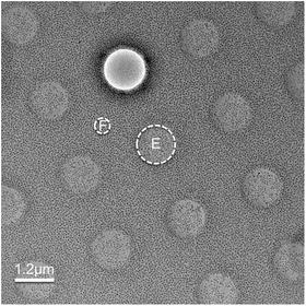
Fig. 1
Low-dose imaging. Shown is a low-mag search mode image of ice-embedded evenly distributed virus particles. The grid carbon bar region (circle with “F” label) will be used to determine focus at high magnification in focus mode. The final image of a hole with particles will be taken in exposure mode (circle with “E”). The grid is a C-flat 1.2/1.3 grid with a hole diameter of 1.2 and 1.3 μm hole spacing
3.7 Data Quantity
The amount of data for different projects is different depending on sample properties (size, symmetry, surface feature, etc.) and targeted reconstruction resolution. For low-resolution (15 Å and lower) 3-D reconstruction, a few hundred icosahedral virus particles are sufficient. Higher resolution reconstruction will need more particles with subnanometer resolution needing a few thousand particles. For near-atomic resolution 3-D reconstructions, about 50,000–100,000 icosahedral virus particles should be imaged. This amount of data is equivalent to about 500–1,000 films (or 2,000–4,000 4K × 4K CCD images) for icosahedral virus of ~50 nm in diameter.
3.8 Image Digitization
For image processing and 3-D reconstruction, the image pixel values should be linear to the density projection of target structures. It is important that the digital images are consistent with this requirement. From electron optics and image formation theory of TEM instruments, the electron wave intensities at the imaging plane are proportional to the structural densities [31] and thus the pixel values for digital camera (i.e., CCD and DDD) images and the optical densities (O.D.) of photographic films (i.e., film darkness) are also linear to the structural densities. The digital camera images can be used as is. However, extra attention should be paid to the photographic films as they must be further digitized using film scanners.
Many different scanners including both commercial products and specially designed scanners have been used in the cryo-EM field [32]. Currently, the most popular scanner is the Nikon Super CoolScan 9000 ED (see Note 4) which scans at 4,000 dpi (i.e., 6.35 μm/pixel). The scanner records the light intensities transmitted through the film and the saved image pixel values are thus the transmittance instead of the optical density values (see Note 5). The scanned images should be transformed so that the pixel values become linear to optical densities. This conversion can be done using the log transform of transmittance.
The convention for image contrast (i.e., brighter or darker pixels for particles relative to background pixels) is different for different image processing software. We adopted the positive contrast convention in which the particles should be brighter in graphic display (i.e., larger pixel values) than the background. The contrast can be inverted by multiplying each pixel value by −1. For CCD images, the contrast needs to be inverted while the scanned image by a Nikon scanner is already in suitable contrast.
The following command will perform image format and O.D. conversion of scanned images (see Note 6):
nikontiff2mrc.py <input.tif> <output.mrc> –ODconversion=<0|1> –invert=<0|1>
The following command will invert the contrast of CCD images:
e2proc2d.py <input.dm3> <output.mrc> –mult=-1
3.9 Image Processing and 3-D Reconstruction
Single particle 3-D reconstructions of icosahedral viruses (see Notes 7 and 8) were among the earliest EM reconstructions of biological structures. Many general software packages or specialized programs have been developed by different groups to perform all or a subset of the image processing and 3-D reconstruction tasks (see http://en.wikibooks.org/wiki/Software_Tools_For_Molecular_Microscopy). Comprehensive coverage of all the software packages is beyond the scope of this protocol. Instead, we will focus on image processing strategies and a set of programs that we routinely use in our projects. We use EMAN [33] and EMAN2 [34] packages as the general image processing software and have developed many additional programs for icosahedral and asymmetric reconstruction of viruses. If not specially explained, in this protocol, the programs starting with “e2” are EMAN2 programs while programs jspr.py, jalign, j3dr, images2lst.py, nikontiff2mrc.py, filterMicrograph.py, goodImageSizes.py, batchboxer.py, fitctf2.py, flipHand.py, commonImages.py, and symreduce.py are developed in the Jiang lab.
As the entire image processing and 3-D reconstruction project consists of multiple tasks in different stages, the protocol is divided into a series of sections in an order parallel to that of image processing tasks carried out in an actual project. Each of the following sections will focus on one of the tasks and the overall image processing strategy will be summarized in the final section.
3.10 Particle Selection
For single particle cryo-EM, the particles in a micrograph must be individually selected and then saved for subsequent processing. While it is possible that particle selection is performed directly from the micrograph of original sampling, we prefer a three-step process that includes prefiltering of micrographs to enhance contrast, particle selection using the prefiltered micrographs, and particle output from original images.
3.10.1 Prefiltering of Micrographs
As cryo-EM images have low contrast due to low-dose imaging and small defocuses, the particles can often be difficult to detect. To enhance the contrast, multiple filtering steps are performed:
Binning. This will remove noises in the high-resolution ranges. Binning also significantly reduces image size and speeds up subsequent selection process. The amount of binning depends on the initial sampling and we typically bin the micrographs by 4–6× so that the virus particle diameters are around 100 or fewer pixels in the binned images.
Low-pass filtering. This further removes noise and enhances the particle contrast. Though the signals at higher resolutions are removed by binning and low-pass filtering, it does not affect particle selection as visibility and localization of particles are based mostly on low-resolution signals.
Gradient removal. This will remove the overall density gradient in the micrograph caused by ice thickness variation, make the contrast of entire micrograph uniform, and eliminate the need of adjusting image display brightness/contrast parameters for different regions of the micrograph.
Removal of pixels with extreme values from X-ray pixels in CCD images or dust on film during scanning. It will help image display with proper brightness/contrast and also improve the robustness of automated particle selection.
The following command will perform these filtering processes with some of the filtering parameters automatically determined using the specified particle diameter and starting image sampling:
filterMicrograph.py <micrographs> –diameter=<Angstrom> –apix=< Angstrom/pixel> –shrink=<n>
3.10.2 Particle Selection
The prefiltered micrograph images are then used for particle selection. The task is to locate good particles that are free of contamination and isolated from neighboring particles (see Note 9). While there are many automated particle selection methods [35], no automated method so far can be fully trusted. In practice, a hybrid approach should be adopted in which manual screening is performed after automated selection.
The selected particles should be well centered to benefit subsequent 2-D alignment steps that determine the particle orientation and center parameters. While automated selection methods in general result in well-centered particles, manual selection often results in particles with significantly more spread of centering. To improve the centering for manual selection, an effective visual guide is to use particle box (or circle if the program allows) about the same size as the virus particle diameter so that the edges of well-centered particles are tangent to the boxes. Off-centered particles will protrude out of the box and can be easily detected by the user (see Fig. 2). Use of this visual guide is facilitated by the separation of particle selection step from output of selected particles. When the two steps are combined in one task, boxes significantly larger than the particles likely lead to poorer centering for manually selected particles. Once the particles in the micrograph are automatically selected and then screened, only the particle locations (i.e., the x, y coordinates for the particle center in the micrograph) need to be saved.
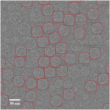
Fig. 2
Particle selection. A typical low-dose image of ice-embedded bacteriophage T7 capsid I particles imaged at 3.0 μm underfocus using a FEI Titan Krios microscope at 300 kV with dose setting at ~25 e/Å2. The red boxes indicate selected capsid I particles. The particles are more packed than optimal distribution but can still be effectively refined with appropriate methods (see Note 9). Contaminant larger capsid II particles and smaller vesicles are not selected since they can be easily distinguished from capsid I particles
The following command will launch the graphic interface for particle selection that supports both automated and manual selection:
e2boxer.py <input filtered micrographs>
3.10.3 Particle Output
The saved particle center coordinates, after being adjusted for the amount of binning in prefiltering, can then be used to “cut” the particles from original micrographs. In this step, the box size can be changed to allow sufficient padding (typically 25–50 %) around the particles. The box size should use a “good” number (see Note 10). Square boxes should be used unless the software explicitly states support for rectangular images. The individual particle images should be normalized (i.e., set mean to 0 and variance to 1) to make particles from micrographs of different ice thickness have similar pixel value ranges.
The following command will “cut” individual particles with particles from the same micrograph saved in same file in HDF format while a separate image file for each micrograph (see Note 6). The particle location and source micrograph are also recorded as metadata in the HDF file.
batchboxer.py <input particle location files> –scale=<n> –removeSpeckle=1 –normalize=1
3.11 CTF Determination
TEM images are modulated by the contrast transfer function (CTF) of the objective lens in TEM optical system [31, 36, 37]. Since the CTF functions cannot be precisely preset and can vary significantly among different images, it is critical to accurately determine the CTF parameters for each micrograph for proper corrections and to reach high-resolution 3-D reconstructions.
Among many of the parameters (defocus, B-factor, noises, etc.), the defocus value (see Note 11) is the most critical parameter to be determined. The signature of CTF is its oscillatory nature [38] which can be seen easily as the Thon rings [39] in the image power spectra (see Fig. 3). The Thon rings oscillate more frequently at larger defocuses and less at smaller defocuses (see Fig. 4). This relationship between defocus and Thon rings is the basis of both manual and automated CTF fitting methods.
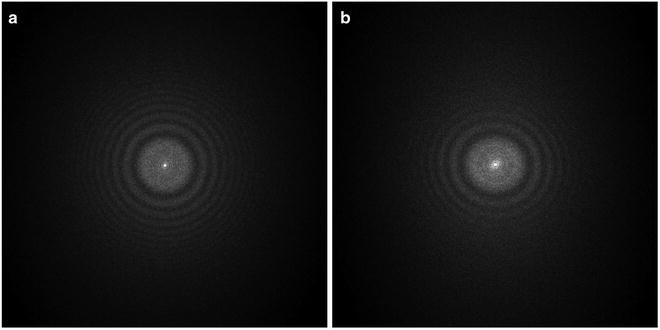
Fig. 3
Image power spectra. (a) Isotropic Thon rings with minimal astigmatism; (b) elongated Thon rings indicating significant astigmatism. The defocus is smallest along the most elongated direction
Fig. 4
CTF fitting. Shown are well-fitted CTF curves of two micrographs with a defocus of 2.1 μm and 0.94 μm, respectively
The image power spectra can be computed from either selected particles [40] or directly from the micrograph using grid boxing [41]. We suggest the former approach as it will enhance the Thon rings by avoiding the micrograph background areas empty of particles. Since the background areas with vitreous ice do not have strong Thon rings, their inclusion will weaken the average power spectra and contribute negatively to the reliability of CTF fitting.
To efficiently process a large number of images needed for high-resolution 3-D reconstructions, we suggest a two-step CTF fitting process that starts with automated fitting [41–46] and then completes with interactive graphic screening/verification. The reason for the need of final manual screening in practice is due to the inevitable occasional failures of automated fitting methods [42] and lack of reliable detection of these failures by the automated methods. In our recent automated fitting method, we have integrated four different automated fitting algorithms which can cross-validate the fitting results and only prompt users with the inconsistent results among the methods for further manual screening [42]. Once CTF fitting is completed, the determined CTF parameters should be saved to the image headers that are needed for subsequent CTF correction and further refinement.
The following commands will perform each of the three tasks:
fitctf2.py <input particle images> –cs=<mm> –voltage=<kV> –apix=<Angstrom/pixel> –oversample=<n>
Interactive screening
fitctf2.py<input particle images>–screenCtf=1
Setting CTF parameters to image header
fitctf2.py<input particle images>–setParm=1
In these commands, we assume that the images are free of astigmatism, which is a reasonable assumption for a well-aligned microscope by experienced microscopists. Though many fitting methods including fitctf2.py are able to determine astigmatism, we typically leave it to later high-resolution refinement steps (see Subheading 3.15). Due to this postponed handling of astigmatism and further refinement of the focus values at the level of individual particles in later high-resolution refinement steps, we typically only record the CTF parameters fitted from power spectra as initial coarse values without CTF phase correction. Instead, CTF correction is performed as part of 2-D alignment and 3-D reconstruction tasks.
3.12 Image Quality Evaluation
Despite careful sample preparation, microscope alignment, and data collection, it is almost always true that the qualities of a subset of images are poor and these images should be discarded. Depending on the type of quality issues, poor quality images can be identified at different steps. For example, during film digitization step, images of very thick ice, large amount of ice contamination, very few particles, or severe charging/drifting do not need to be scanned. However, stringent image quality evaluation is generally evaluated using the image power spectra and often integrated as part of the manual screening/verification of fitted CTF parameters.
A high-quality image should have isotropic Thon rings in its 2-D power spectra and the Thon rings should extend to high resolutions (i.e., closer to the edge of 2-D power spectra). Elongated Thon rings indicate a significant level of astigmatism (see Fig. 3). Astigmatic images should be discarded if the image processing and 3-D reconstruction software does not support determination and correction of astigmatism. In the image processing strategy described here, astigmatic images can be effectively utilized. When the Thon rings are significantly weaker along some direction than its perpendicular direction, the specimen has undergone significant drift or charging during exposure. These images should be discarded. Sometimes, a sharp peak can be seen at 3.7 Å in the 1-D power spectra, which is indicative of a significant level of ice contamination. Occasionally, we have also seen sharp peaks in the power spectra which were ultimately traced back to a malfunctioning scanner.
The Thon rings gradually become weaker at higher resolutions and the rate of weakening can be used to quantify the image quality. The quality factor is termed as B-factor (see Note 13) of which the value can be obtained during CTF fitting [40]. Smaller B-factors correspond to better quality images and B-factors of low-dose cryo-EM images of biological samples taken with modern TEMs with a FEG gun can reach values around 200 Å2 or better. Studies of B-factor distributions have found that B-factors become slightly larger at large defocuses [40], so it is beneficial to collect images at smaller defocuses. In consideration of decreased image contrast at a smaller defocus, a defocus range of 1–2 μm should be a good compromise of the different factors for near-atomic resolution 3-D reconstruction of many viruses.
It is often observed that the image qualities can vary significantly even among images taken in same session. It is common practice to only select the best fraction of the images for inclusion in further image processing and 3-D reconstruction. The selection can be done using a graphic CTF fitting program such as ctfit in EMAN to examine the resolution of the last visible CTF peaks in the 1-D power spectra plot (see Fig. 4 and Note 14). Depending on the goal of the project, the resolution limit should be adjusted accordingly. For example, only images with CTF peaks beyond 6 Å will be included for projects aiming at near-atomic resolution (3–4 Å) reconstructions. However, it must be pointed out that the visibility of CTF peaks at high resolution is affected not only by imaging quality but also by other factors and the resolution cutoff should not be overly aggressive, especially for near-atomic resolution projects. For example, a small number of particles in a single micrograph might not have sufficient scattering power for clearly visible CTF peaks at high resolutions. Another common reason is the focus variations due to either residual astigmatism, small local tilt of the sample, or simply the particle Z-position variations in thick ice. Averaging of the power spectra of different focuses will effectively accelerate the apparent decay rate of CTF peak heights and even introduce zero CTF peak heights at a certain resolution beyond which weak CTF peaks become visible again [47]. These second groups of CTF peaks are out of sync with the first group of CTF peaks at lower resolutions, and their peak positions cannot be simultaneously fitted with a single defocus. These focus variations can be effectively determined and corrected with proper 2-D alignment methods (see Subheading 3.15). From these analyses and experiences with many datasets, we suggest that cryo-EM image qualities are often better than what the highest resolution CTF peaks or the fitted B-factors indicate. It is now a common observation that 3-D reconstructions can reach a resolution significantly beyond the apparent limit of the images.
The particle images that pass the quality screening are deemed good and will be included for subsequent image processing and 3-D reconstruction. All these particle images can be pooled into a single large dataset using the following command:
images2lst.py<input image files><output data set.lst>
3.13 Initial Icosahedral Model
As single particle cryo-EM images are 2-D projections of the to-be-determined 3-D structure at random views, the inverse problem is to determine the 3-D structure from these 2-D images using computational image processing methods. Current image processing methods rely on iterative processes in which the 3-D reconstruction is iteratively improved. It is critical that the initial 3-D model is correctly constructed before proceeding to full refinement. If an initial model is already known from earlier studies of the same virus or its homolog, that initial model can be used (see Note 15) and the user can skip the step on building the initial model in this section. For a project on a new virus structure, several methods have been developed in the field to build a de novo initial model:
Self-common line method. This is the classic method that takes advantage of the icosahedral symmetry of many virus structures. Based on Fourier central section theorem [48], the 2-D Fourier transform of a projection image is equivalent to a central section of 3-D Fourier transform of the original 3-D structure and the central sections of different views intersect at a common line through the Fourier origin [49–51]. Due to icosahedral symmetry, the symmetry-related views of the same particle can have up to 37 pairs of common lines, which are often termed as self-common line (see Note 16). The unique property of this method is that the information from a single image is self-sufficient to determine the particle orientation without need of a reference. The weakness of this method is that the common lines are clustered for views near symmetry axes that introduce biases [52]. This method also only works well for images with large defocus values and good contrast, which was the underlying need for a focal pair imaging strategy, often used in the past [51]. We now seldom use this method.
Symmetry view method. This EMAN method intentionally searches for particle images with best five-, three-, and twofold symmetry characteristics and uses these particles to construct the first crude 3-D model that will be further refined. This method is available in the EMAN program starticos.
Synthetic model method. An icosahedral shape geometry can be computationally synthesized that approximates the size, angularity, and shell thickness of the target virus based on visual information from the particle images. We implemented this method via the processes mask.icos and mask.dodecahedron that can be executed via e2proc3d.py program.
Random de novo model method. In this method, random orientation parameters (i.e., Euler angles; see Note 17) are assigned to the particles for reconstruction of the initial 3-D density map model. Since the view parameters are random, the initial model is essentially a spherical average without any meaningful surface features. However, the model does reflect the average size and shell thickness of the viral structure which are often sufficient for subsequent iterative refinements to converge to correct structure (see Fig. 5) [53, 54]. This is our preferred method for building initial model.
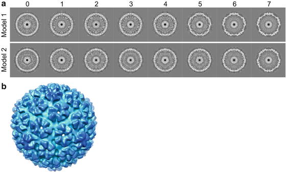
Fig. 5
De novo icosahedral reconstruction initial models. (a) Shown are the convergence histories for two random initial model refinements for bacteriophage T7 capsid I. The numbers at the top are the refinement iterations. The initial icosahedral model (iteration 0) was built using randomly assigned particle orientations. The two de novo models with opposite handedness illustrate that single particle cryo-EM 3-D reconstruction cannot uniquely determine the absolute handedness. (b) The threefold surface view of model-1 that is radially colored
In this protocol, we will focus on the random de novo model method. In general, only a small dataset at coarse sampling (via binning of the particle images) is needed for building the initial model. We typically bin the images 4× so that the sampling of the binned images is around 4–6 Å. The binning not only reduces the image size to speed up computation but also effectively enhances the image contrast for more robust initial model building. The following command will bin the images:
e2proc2d.py<input particle file><output particle.hdf>–meanshrink=<n>
A small number of particles (100–200) randomly selected from the entire dataset are typically used for initial model building:
images2lst.py<whole dataset.lst><subset.lst>–randomSample=<n>
Particles of homogenous conformation and good contrast will enhance the success rate of the random de novo model method. If the quality or contrast of the randomly selected particles consistently cause initial model building to fail, the user can manually screen the particle images and select particles at larger defocuses and with higher contrast. This can be done by running
to display the particles and then using the “Sets” tab function in its control widget.
e2display<whole dataset.lst>
The random de novo model construction and refinement can then be performed using the following command:
jspr.py <particles.lst> –nRepeat=<n> –sym=icos –diameter=<Angstrom> –apix=<A/pixel> –iters 8 –cpus=<n>
As the random de novo model method starts from random parameters and some of the starting points might be too distant for the iterative refinements to converge to the correct solution, it might be necessary to repeat the random de novo model method multiple times (with different random initial views assigned to the particles) to obtain a correct initial model. The parameter –nRepeat=<n> can be used to specify the number of repeats. The multiple independent de novo models are also useful for removing bad particles in subsequent full dataset refinement (see Subheading 3.14).
In single particle cryo-EM, the image processing programs can always produce 3-D density maps, though currently no method can either guarantee that these density maps are correct models or offer a score to accurately quantify the reliability of the models. However, for a new project with a completely unknown target structure, a critical decision on whether the model is correct must be made. Here, we list a few criteria that can help make the decision:
Consistent models (ignoring potential difference in handedness; see Fig. 5 and Note 18) from multiple random de novo model processes.Related posts:
 Microwave-Assisted Processing and Embedding for Transmission Electron Microscopy
 Electron Microscopy of Microtubule Cytoskeleton Assembly In Vitro
 Biological Applications of Energy-Filtered TEM
 Freeze Fracture and Freeze Etching
 Elemental and Isotopic Imaging of Biological Samples Using NanoSIMS
 X-Ray Microanalysis in the Scanning Electron Microscope

Stay updated, free articles. Join our Telegram channel

Full access? Get Clinical Tree


