and Jeremy A. Shaw1
(1)
Centre for Microscopy, Characterisation and Analysis, The University of Western Australia, Crawley, WA, Australia
Abstract
The techniques of electron energy-loss spectroscopy (EELS) and energy-filtered TEM (EFTEM) are routinely applied in the physical sciences to map the distribution of elements at the nanoscale. EELS can also provide details of the bonding/valence of elements through variations in the fine structure of elemental peaks in the spectrum. While applications of these techniques in biology are less prevalent, their ability to detect both the light elements (e.g., C, N, O, P, S) that form the building blocks of biological systems and heavier elements (e.g., metals) makes them potentially important techniques for investigating local chemical variations in tissues and cells. Successful application of EELS and EFTEM in biology requires both an understanding of the techniques themselves and expertise in specimen preparation. Care must be taken to avoid the diffusion of elements during the preparation process to avoid artifacts in the resulting element maps. The power of the techniques is demonstrated here using tissue from a marine mollusc (chiton).
Key words
Transmission electron microscopyElectron spectroscopyCompositionElemental mapping1 Introduction
The twin techniques of electron energy-loss spectroscopy (EELS) and energy-filtered transmission electron microscopy (EFTEM) provide information on the presence and distribution of elements and can be used to investigate the form of those elements, e.g., their bonding, valence, and coordination [1–4]. They are extensively used in the physical sciences, where they routinely provide compositional and electronic information down to the nanoscale and, on the latest-generation instruments, at near-atomic resolution [5]. Applications of EELS and EFTEM in biology are, however, less widespread, in part due to the tendency for the necessary instrumentation to be located in materials science and engineering departments from which biologists are often excluded, but also because of the increased complexity of applying these techniques in biological research. The potential benefits of the techniques in biological research are, however, significant as they are capable of detecting the light elements central to biology, e.g., C, N, O, P, and S [6–10], in addition to key metals related to biological function, e.g., Fe and Ca [11–17], and the broad spectrum of elements arising from nonbiological materials introduced into biological systems either intentionally or unintentionally [18, 19]. This potential can be demonstrated by analyzing the composition of tissue from a marine mollusc (chiton), which hardens its teeth with iron and calcium mineral phases. This is achieved by transporting large quantities of iron into the teeth from stores of ferritin within the surrounding tissue. The ferritin is aggregated into siderosomes containing thousands of individual ferritin molecules, each with an iron core of ferrihydrite ~8 nm in diameter (see Fig. 1). This complex biomineralization system results in a laminated biocomposite structure comprised of iron oxides, iron hydroxides, and calcium phosphate, with the exact structure/phases dependent on the species [12–14, 16].
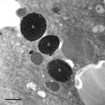
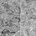
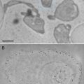
Fig. 1
Bright field TEM image of superior epithelial tissue from the marine chiton Acanthopleura hirtosa (Mollusca: Polyplacophora). The superior epithelium is responsible for hardening the animal’s teeth with iron biominerals. Iron is stored in the tissue as ferritin, which aggregates into large electron dense siderosomes (S), prior to delivery into the teeth. Scale bar = 500 nm
EELS involves the analysis of the energy lost by electrons passing through a thin section. An energy-loss spectrum is formed by collecting these transmitted electrons and physically dispersing them as a function of their energy, typically using a magnetic prism (or multiple prisms). To acquire EELS data, you will need either a dedicated electron spectrometer or an energy filter that allows both imaging and spectroscopy. The filter can either be built into the microscope column just below the objective lens (an in-column filter) or attached to the bottom of the TEM after the projector lens system (a post-column filter). The former design (available for Zeiss or JEOL TEMs) must be included in the microscope design at construction. The latter (available from Gatan) can be retrofitted to any TEM.
In a thin sample, the EEL spectrum is dominated by a large peak at zero energy loss representing the electrons that pass through the specimen with no significant loss of energy (the elastic scattered electrons). In the so-called low-loss region of the spectrum (the first few tens of eV energy loss), the main signals are the broad plasmon peaks corresponding to collective vibrations of the valence electrons in the specimen (see Fig. 2a). Weak signals associated with the excitation of chromophores have been analyzed in special cases [20], but applications in this area are rare.
Fig. 2
Electron energy-loss spectra. (a) Low-loss spectrum from the field of view shown in Fig. 1 showing the dominant zero-loss peak (at 0 eV) and plasmon peak (at ~20 eV). (b) Series of core-loss edges from C, N, O, and Fe from the same chiton sample. The energies of the peaks determine which elements are present while the fine structure can reveal information on the local bonding environment, e.g., valence or oxidation state
Of most interest for biological research are the core-loss signals, which provide information on specific elements. The core-loss signals are associated with electrons being excited from inner (core) electron shells into the outer (valence) shells of the atoms in the specimen. They occur at characteristic energies for each element (approximately the element’s ionization energies) and have a fine structure that is representative of the form of the element, e.g., its valence/oxidation state, bonding environment, and coordination (see Fig. 2b).
In EELS, a spectrum showing the number of electrons as a function of energy loss is acquired, allowing the elements present to be identified from their characteristic energies and details of the elements’ state to be determined from the fine structure [2]. In EFTEM, images are formed at user-defined energies by using an energy-selecting slit to define the energy range of the electrons forming the image while filtering out the unwanted electrons. By selecting the energy range corresponding to a specific element, the distribution of a given element can be directly imaged in the form of an element map.
These elemental signals sit on a background signal created by energy-loss events at lower energies, i.e., plasmon peaks and lower-energy element peaks. The elemental signal can be separated from the background by fitting a suitable function through the pre-edge background data. For EFTEM element mapping, this is typically done using the three-window method [1] where two background (or pre-edge) images are acquired at energies just below the characteristic element energy and a third image (the post-edge image) is acquired above the characteristic element energy (see Fig. 3). The two pre-edge images are used to fit a background function allowing extrapolation of the background to the post-edge energy and the removal of the background intensity. If the background can be accurately removed, the final element map will contain quantitative intensity variations corresponding to the distribution of the element (number of atoms per unit projected area). An example of this three-window approach for the mapping of iron in the chiton tissue is shown in Fig. 4. The two pre-edge images are acquired at energies of 645 ± 20 eV and 685 ± 20 eV, while the post-edge image is acquired at 735 ± 20 eV, slightly above the onset of the Fe L2,3 edge. The resulting element map clearly shows the iron distribution in the tissue.
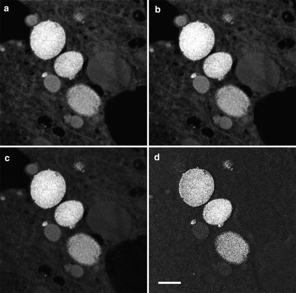
Fig. 3
EELS spectrum showing the O and Fe core-loss edges along with the location (for Fe) of the two pre-edge and post-edge energy windows used to acquire the three images in the three-window technique. The final element map is obtained by fitting a background from the two pre-edge images and extrapolating and subtracting that background from the post-edge image (see Fig. 4)
Fig. 4
Application of the three-window technique to map the iron distribution in ferritin accumulated in the chiton tissue. (a–c) Pre- and post-edge images for the Fe L2,3 edge centered at 645 eV, 685 eV, and 735 eV, respectively, with a energy window of 40 eV. (d) Resulting Fe element map once the background has been removed from the post-edge image. Scale bar = 500 nm
For some elements, multiple signals at different energies may be detectable by EELS. In the case of Fe, in addition to the L-edge used to create the map in Fig. 4, an M-edge can be found at ~54 eV. The choice of which peak to map can often be difficult. Higher intensity levels (and hence better signal-to-noise and shorter acquisition times) are associated with lower-energy edges. Signals close to the dominant plasmon peaks in the low-loss region of the spectrum are, however, difficult to map accurately due to problems fitting appropriate background models to extract the elemental signal. While we have successfully mapped Fe using the M-edge in very thin sections, where the plasmon peaks are less significant, for more conventional section thicknesses, the higher energy L-edge produces more reliable results.
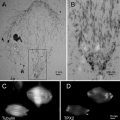
The ability of EFTEM to acquire multiple element maps, including key biological elements such as C, N, and O, is illustrated in Fig. 5, where a set of element maps acquired from the same field of view is shown. In each case, the energy range for each of the pre- and post-edge images has been optimized using the spectral data shown in Fig. 2b, and the acquisition times have been adjusted to provide good signal-to-noise (from 120 s per image for C up to 240 s per image for iron).
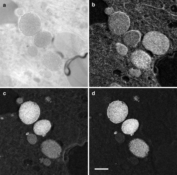
Fig. 5
Comparable element maps for (a) carbon, (b) nitrogen, (c) oxygen, and (d) iron from the same field of view as shown in Fig. 1. Scale bar = 500 nm
In situations where it is difficult to fit a suitable background, e.g., where multiple signals overlap, the jump ratio imaging method may be more useful. In this case, only two images need to be acquired, the post-edge image and one pre-edge image. The jump ratio is produced by dividing the post-edge image by the pre-edge image. The resulting image will show higher intensity where the element is located, but the resulting data is only a qualitative indication of the element distribution. Jump ratio imaging has fewer problems with noisy data as it does not require the fitting of a background function. For many biological EFTEM applications, obtaining high signal-to-noise is problematic as element concentrations can be low and beam damage limits acquisition times. Thus, jump ratio imaging is often a preferable alternative to the full three-window element mapping technique.
In all cases, it is advisable to acquire electron energy-loss spectra from the specimen before conducting energy-filtered imaging. It is only the presence of the elemental signature in the spectrum that provides proof that the element is present. EFTEM techniques are prone to weak artifactual intensity variations created by fluctuations in the background. Thus, a low-intensity false-positive result can occur in situations where the element is not present, and it is only the spectral confirmation that provides evidence of the element’s presence. A second reason for acquiring representative spectra is that this allows for the optimization of the energies of the signal and background windows used to form the image. By ensuring that the post-edge window is positioned on a strong feature in the elemental signal, good signal-to-noise will result in the final image [21]. A basic procedure for the acquisition of an EEL spectrum suitable for the optimization of the pre- and post-edge windows for EFTEM is provided in Subheading 3.2.
An alternative to element mapping by energy-filtered TEM is to acquire EEL spectra as a function of position by running the microscope in Scanning TEM (STEM) mode and acquiring a full spectrum at each point in the scan. This generates a data cube with two of the dimensions representing the position of the electron beam as it is scanned and the third dimension representing the energy lost by the electrons. This data cube can be post-processed to extract the elemental information as a function of probe position. This has the advantage that the presence of the element is confirmed through its appearance in the spectrum and that both the location and electronic state, e.g., valence/oxidation state, of the element can be mapped [22]. Acquiring the full data cube also allows for the data to be interrogated and elements to be identified and mapped long after the data is acquired (unlike EFTEM where specific acquisition conditions must be set up for each element we wish to analyze at the time of data acquisition). The disadvantages are that longer data acquisition times are required compared to EFTEM and that the technique is more technically demanding and complex.
As EELS and EFTEM rely partly on the assumption that the target material is of even thickness, analyses of biological material are best conducted on resin-embedded samples cut with an ultramicrotome. Conventional benchtop and microwave-assisted chemical fixation and cryogenic methods can be used successfully for preparing embedded biological samples for EELS and EFTEM (see Chapters 1, 2, 3, and 8 of this volume). However, a number of provisos exist when the target of the preservation is to capture the elemental composition rather than pure structure. Certain elements, whether they exist as mobile ions or are bound to cellular components, can be moved, lost, or changed during the various processing steps. As such, a thorough understanding of the sample’s chemistry is required, together with the specific interactions that may occur between the target elements and their exposure to the chemicals necessary for preparing material for TEM. Often, a compromise must be made between the good structural preservation that can be achieved with routine TEM sample preparation and protocols that aim to preserve the qualitative or quantitative elemental composition. No single protocol exists, as the method is dependent on the sample, the target element, and how this element is integrated into the tissue. For a detailed overview of the specific considerations needed for biological microanalysis, we recommend [23, 24].
High-pressure freezing (HPF) is a reliable method for preserving the structural and elemental composition of cultured cells or whole tissues. This is followed by freeze-substitution of the sample, which can be loosely defined as a low-temperature dehydration technique. The freeze-substitution solution uses an organic solvent containing a range of additives (e.g., uranyl acetate, osmium tetroxide, and water), which act as fixatives and contrast agents to biological tissues for structural imaging in the TEM. Care must be taken when preparing the freeze-substitution medium to exclude elements that may share characteristic peaks with target elements for analysis (e.g., the low-energy edges of Os and U interfere with our ability to map the Fe M-edge or the Au O-edge). It is possible to omit any or all of the additives from the organic solvent; however, this commonly compromises the samples structural preservation. In this case, it is recommended that suitable duplicate samples are processed for comparative structural observations. Although freezing circumvents issues relating to the extraction or displacement of elements in biological samples, it must be stressed that subsequent freeze-substitution, resin embedding, and cutting of ultrathin sections on water can each result in element loss and/or redistribution. For further reading we recommend [25]. In some instances, cryo-ultramicrotomy of frozen hydrated material and subsequent freeze-drying of the sections may be applicable. While this may improve the retention of elements, the removal of water will result in uneven sample thickness.
2 Materials
2.1 Specimen Preparation
3.
Extracellular filler (such as 1–2 % low gelling temperature agarose or 10–20 % bovine serum albumin). For assisting the freezing process (see Note 2).
4.
Sample holders. As per brand/model of high-pressure freezer.
5.
Micropipette and tips (0.1–2.5 μL and 2–20 μL). For transferring filler and/or samples into sample holders.
6.
Dry block heater and temperature-controlled microscope stage (set to ~37 °C range). Important if using agarose to prevent it from cooling below its gelling temperature during sample loading. Agarose must be kept as a liquid until the point of freezing.
7.
Cryovials. For storing frozen samples or conducting the freeze-substitution process.
9.
 Microwave-Assisted Processing and Embedding for Transmission Electron Microscopy
 Electron Microscopy of Microtubule Cytoskeleton Assembly In Vitro
 Visualization of DNA and Protein–DNA Complexes with Atomic Force Microscopy
 Biological Applications of Phase-Contrast Electron Microscopy
 Correlative Light and Electron Microscopy Using Immunolabeled Sections
 X-Ray Microanalysis in the Scanning Electron Microscope


Resin embedding media. Used as part of an increasing concentration series to infiltrate the cells/tissue prior to polymerization and sectioning (see Chapter 1 of this volume for details). The resin should be free of any elements that are intended for analysis. Epon 812 (Procure 812) or Lowicryl HM20 is recommended for most samples.
Related posts:
Microwave-Assisted Processing and Embedding for Transmission Electron Microscopy
Electron Microscopy of Microtubule Cytoskeleton Assembly In Vitro
Visualization of DNA and Protein–DNA Complexes with Atomic Force Microscopy
Biological Applications of Phase-Contrast Electron Microscopy
Correlative Light and Electron Microscopy Using Immunolabeled Sections
Stay updated, free articles. Join our Telegram channel
Full access? Get Clinical Tree
