12 Specimens and Technique

Using specimens from the neuroanatomical collection of the Hannover Medical School the authors have been able to gain valuable information about the sectional anatomy of the head and variability of neuroanatomical structures. This collection comprises 35 intracranially fixed brains of deceased individuals who bequeathed themselves for teaching and research at the Center for Anatomy of the Hannover Medical School. In addition, the collection contains serial neurohistological sections from 34 brains that were fixed after removal.

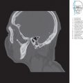
All illustrations in this atlas have been largely depicted with the aid of original sections; axial illustrations were based on corresponding MR and CT images except the brainstem series. The original specimens for the illustrations were obtained from three deceased individuals and those for the axial imaging from one subject; age, sex, length, head measurements, and possible cause of death of these four subjects have been listed in ▶Table 12.1. The maximum width of the head was measured above the external acoustic canal, while its maximum length was measured between the glabella and opisthion. Facial height was measured between the nasion and gnathion and the width of the zygomatic arch was measured between the most lateral points of the zygomatic bones. Serial CT images of the skull base were obtained retrospectively from a diagnostic examination of a 32-year-old male patient with no available details about cranial parameters. CT images aligned along the supraorbito-suboccipital plane were also obtained retrospectively from a diagnostic examination of a 64-year-old female patient.

Cerebrospinal fluid of the corpse was drained by suboccipital and lumbar puncture, and the same amount of 37% formalin (Merck) was injected into the subarachnoid space. A fixation mixture of 86 parts 96% alcohol, 8 parts 37% formalin, 3 parts glycerin DAB 7, and 3 parts saturated phenol solution DAB 8 were perfused through the femoral artery.

MR images of the test subject were obtained conforming to coronal, sagittal, and brainstem series, which closely approximated atlas illustrations. Sectional planes were specified in accordance with stereotactic principles. These coordinate planes have been described earlier in ▶Section 1.2 for coordinate systems oriented in the coronal, sagittal, and axial planes together with a description of the Meynert plane, which was employed in the coordinate system of the brainstem series.

The corresponding coordinate planes must be visible on individual cranial sections such that these sections may be spatially oriented in the coordinate system. Thus, corresponding coordinate planes, such as the median plane, Reid’s baseline, the meatovertical plane, and Meynert’s plane, were marked on the head using deep, circular incisions which later served as orientation for individual cranial sections, thereby enabling correct alignment of these sections within the coordinate frame.

These heads were subsequently frozen at −26°C for 6 days and then cut through using a KS 400 band saw (Reich, Nürtingen). A special guide was then used to obtain sections at 10 mm intervals while brainstem sections were obtained at intervals of 5 mm. Sawing reduced the thickness of each section by 1 mm.

The cut surfaces of these sections were photographed and photo prints were obtained on a scale of 1:1. Illustrations were made with acetate overlays and permanent ink directly from photographs while comparing them throughout with original preparations. Individual structures were identified using a Zeiss stereomicroscope together with a Volpi cold light source Intralux 150 H. Gennari’s band in the primary visual cortex, the corona radiata, and the alveus of the hippocampus were thus easily identifiable in the alcohol-formalin fixed brain slices. Small vessels were examined to histologically differentiate them into arteries or veins. Serial sections of neuroanatomical specimens at the Hannover Medical School were used for histological comparison. Furthermore, one of the authors (H.-J. K) studied the brains of the Yakovlev collection at the Walter Reed Hospital in Washington, D.C., for comparative purposes with a financial grant from the German Research Society (Kr 289/15). A digital drawing board was used to make schematic diagrams of axial sections oriented along the bicommissural plane based on the respective section.

Individual gyri and sulci of the cerebral hemispheres could only be identified with certainty after 1:1 brain models or plexiglass reconstructions were prepared and compared with a series of macroscopic sections from other brains and heads. Reconstructions of T1- and T2-weighted 3D data sets as well as venous and arterial MRA were used for anatomical mapping of MRI images.

Toward the final phase of investigation, the authors (H.-J. K., W.W) assembled cranial sections for the precise localization of sectional planes on radiographs.

To compensate for the 1 mm loss in thickness of the slices due to the width of the blade (approximately 14 mm for 14 sections), the radiographs were cut into strips corresponding to slices and remounted with a 1 mm space between each individual slice. ▶Fig. 3.1c, ▶Fig. 4.1b, and ▶Fig. 5.1b were obtained in this way. Medial and lateral views of the brain (see ▶Fig. 3.1c, ▶Fig. 3.1d, ▶Fig. 4.1c, ▶Fig. 4.1d, ▶Fig. 5.1c, and ▶Fig. 5.1d) were obtained after a midline incision through sections of the brain with the freed halves being assembled into a complete hemisphere or brain. These were photographed, and the missing 1 mm intervals were compensated for. A computerized graphic reconstruction of the lateral view of the ventricular system (see ▶Fig. 7.8b and ▶Fig. 7.11b) was obtained using these slices (program by Dr. B. Sauer), and topographically superimposed within the outlines of the radiographic image of the cranium (see ▶Fig. 3.1c and ▶Fig. 5.1b).

The small cerebral arteries running within sulci of the cerebrum are often very tortuous and have many branches. The course of these fine arteries could not be reconstructed with certainty on 1-cm-thick sections. Therefore, when referring to these branches of the anterior cerebral artery the precuneal artery is meant in general without attempting to differentiate between superior and inferior precuneal arteries. Similarly, temporal and parietal branches of the middle cerebral artery are not subdivided further. Small arteries running entirely within a slice parallel to the sectioning plane have not been sectioned and have therefore not been depicted in the illustrations.

Graphic illustrations in the atlas were reduced in size for printing; coronal series (see ▶Fig. 3.2 to ▶Fig. 5.15) to 82%, sagittal series (see ▶Fig. 4.2 to ▶Fig. 4.7) to 71%, and the overall view of the brainstem series (see ▶Fig. 6.4a to ▶Fig. 6.13a) to 79%. The scale, in centimeters, may be read from the corresponding coordinate frame in the atlas illustrations of the coronal, sagittal, and brainstem series.

Serial MR and CT images of the brainstem series were acquired in coronal and sagittal planes in close approximation to the illustrations in the anatomic atlas. Sectional planes used in digital imaging were aligned with utmost care with anatomical sections. The most representative of several MR and CT images was placed next to atlas illustrations. MR images were obtained from a 33-year-old man. The MR examinations were carried out over several days on a Magnetom Verio 3T, a magnetic resonance tomograph (Siemens, Erlangen), using a 32 channel head coil. Measurement parameters for MR images were selected for acquisition and description of brain anatomy. The spatial relationship of individual structures to anatomically adjacent structures in the same section as also to those in adjoining slices may help delineate their morphology.

The best possible depiction of neuroanatomical structures for the selected examination sequence and window settings with good differentiation of gray and white matter was the main idea behind this book. Bones, muscles, tendons, and fat must remain discreetly in the background.

All T1-weighted MR images in the atlas were obtained with a T1-weighted gradient echo–FLASH sequence. A T1-weighted SE sequence was employed for imaging stages of brain maturation (see ▶Table 12.2 for measurement parameters). T2-weighted images of brain parenchyma were obtained using a TSE sequence. Other special sequences for various regions (DTI, QSM, high resolution images of the petrous bone) have been listed in ▶Table 12.2.

The QSM method is an advancement of SWI technology, whereby phase-shift information of MR signals are calculated and included into the image; substances with paramagnetic properties appear bright, while substances with diamagnetic properties appear dark. The so-called MEDI method was used in the calculation of the QSM image^{660 , 661} for ▶Fig. 7.45, using SWI images with varying echo times. A 3D time-of-flight sequence was used for the 7-T-MRA (see ▶Fig. 7.27) of a 26-year-old, healthy volunteer provided by Dr. Wrede (Essen) (pixel size: 0.22 × 0.22 × 0.41 mm²⁷⁶). For the 7-T image of the hippocampus of a 38-year-old healthy volunteer provided by PD Dr. Theysohn (see ▶Fig. 3.9f), a T2-weighted TSE sequence with a resolution of 0.25 × 0.25 × 3.0 mm was obtained (echo time: 95 ms, repetition time: 5,000 ms, flip angle: 150°, and parallel-imaging factor: 2). The 7-T-SWI image of the deep and basal veins provided by Dr. Deistung (Jena) (see ▶Fig. 7.36e) is a 2-cm-wide minimum-intensity projection (MinIP) of an SWI measurement with 3D flux compensation (echo time: 10.5 ms, repetition time: 17 ms, flip angle: 8°, matrix: 576 × 414 × 256, and voxel size: 0.4 × 0.4 × 0.4 mm). Data were collected in three different head angle positions relative to the direction of the B0 field, and information was combined into a single image. Image contrast in this technique is based on a pronounced sensitivity of this sequence for disturbances of the magnetic field; signal loss within veins results from paramagnetic effects of deoxyhemoglobin.

The 7T-tractography images (see ▶Fig. 7.54d, ▶Fig. 7.54f, and ▶Fig. 7.54g) were derived from a healthy volunteer using a 7T Magnetom MR scanner (Siemens Helathineers, Erlangen, Germany) with a strong gradient system (Siemens SC72, gradient amplitude 70 mT/m, slew rate 200 T/m/s), a 24-channel headcoil (Nova Medical, Massachusetts, USA) and a single refocussed spin-echo EPI sequence (voxel size 1 × 1 × 1 mm, b = 1000, 60 diffusion directions, TE = 67 ms, TR 11, 2s, parallel imaging factor 3, band with 1089 Hz/pixel; 4 measurements). The diffusion data were corrected for motion artifacts and noise, the images were calculated using a deterministic tractography algorithm.

The reader’s attention is drawn to the fact that the specimens for atlas images for the frontal, sagittal, and brainstem series was derived from three different individuals (see ▶Table 12.1). MR images aligned along coronal, sagittal, and bicommissural planes, as well as those of the brainstem series have all been derived from one individual. The other MR and CT images in this book were obtained from different individuals. These interindividual differences in anatomic structures correspond with variations seen in routine clinical practice. Considerable anatomic variants and intracranial mass displacements were disregarded since the authors’ aim was to depict “normal” neuroanatomy, thus enabling identification of pathological changes.