- Cell survival curves and how they are obtained
- The significance of the two portions of the survival curve
- Effects of different radiation conditions, type, and oxygen on the shape of the survival curve
- The relationship between cell repair and the shoulder region of a survival curve
- Common mathematical models used in analyzing cell survival curves and the key parameters associated with each model
- Clinically important radiosensitizers and radioprotectors
Introduction
A cell survival curve is a plot of the number of cells that survive to form colonies as a function of radiation dose. Thus, cell survival curves measure reproductive cell death. Some damaged cells may continue to function for a time, but if they do not reproduce, they are not counted as survivors.
In a cell survival experiment, cells are seeded onto petri dishes and exposed to various doses of radiation. The number of cell colonies that subsequently grow is determined. Each colony is assumed to be derived from a single surviving cell. A cell survival curve is a plot of the fraction of cells that survive (normalized by the fraction of cells that survive with no radiation exposure) versus the radiation dose; each point on a cell survival curve corresponds to a single dose of radiation. Usually, the log of the surviving fraction is plotted on the vertical axis versus dose on the horizontal axis. Mammalian cell survival curves generally show an exponential response to high doses of radiation with a “shoulder” of varying widths in the low-dose range. The effect of radiation on cells can be observed by noting how the cell survival curve changes under different conditions. These changes in condition include using different types of radiation, changing the environment, adding or subtracting oxygen, or delivering the radiation at different times or during different parts of the cell cycle. The study of survival curves revealed many aspects of radiation damage long before the structure of DNA was elucidated.
The In Vitro Survival Curve
“In vitro” means outside a living organism—for example, in a test tube or petri dish. Cell survival can be defined in terms of the reproductive ability of the cells; that is, cells that cannot reproduce are effectively dead. This definition makes sense in the context of common laboratory experiments used to study the effects of radiation on cells prior to the 1980s, when DNA probes began to be available. Cells that continue to reproduce (in petri dishes in the lab) form colonies that are visible to the naked eye, and it is easy to count the surviving colonies after irradiation. This experimental design made it possible to establish many basic facts regarding radiation effects on cells in the early days of radiobiology. By varying the conditions during and after exposure, the factors influencing cell response to radiation can be isolated and studied. The shape of the survival curve contains information regarding the overall sensitivity of the cells, as well as the ability of the cells to repair and recover from radiation damage. Theoretical models have been developed to explain the shapes of the resulting survival curves in terms of cell survival characteristics.
Although reproductive capacity is a good way of defining “cell survival” in the context of in vitro radiobiology experiments, it is not applicable to all cell types. Some cells such as nerve, muscle, and secretory gland cells are nonproliferating. For these cell types, what matters to an organism exposed to radiation is whether the nonproliferating cells maintain function. For proliferating cells (e.g., intestinal lining, stem cells, cells in a cancerous tumor), the reproductive capacity is important, in both the organism and in the laboratory. Reproductive capacity is also referred to as “clonogenic potential.”
The loss of clonogenic potential is a very narrow definition of cell death. A cell that is exposed to radiation may be apparently intact, it may synthesize protein/DNA, and it may even carry out several cycles of mitosis; but if it cannot carry out sustained replication, then it has not survived, according to the definition here.
Cell Survival Curves: Description of Experimental Method
Cell cultures are generated by extracting live cells from various species of mammals such as mice, rats, or humans. The cell population is first grown in a tissue culture flask. The cells are then released from the flask by adding trypsin, the cells are counted, and then a known number of cells is plated onto growth medium in a petri dish and maintained under appropriate conditions (correct temperature, atmosphere, nutrient levels) to survive and grow.
In order to study radiation effects on the cells, many petri dishes are plated under the same conditions using genetically identical cells. Some dishes are not irradiated and are maintained as controls, and the rest of the dishes are exposed to various doses of radiation. The irradiated cells and control cells are then incubated for some time (e.g., a few days up to a couple of weeks) to allow colonies to arise from the surviving cells. A colony is assumed to form by the sustained proliferation of a single cell. Figure 5.1 illustrates a typical cell survival experiment. Here, populations of identical cells are irradiated with increasing doses of radiation.
Figure 5.1 Survival curves are generated by irradiating populations of genetically homogeneous cells with increasing doses of radiation. A plot of the surviving fraction as a function of dose is known as the cell survival curve.
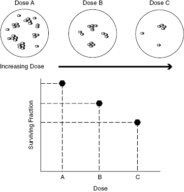
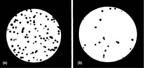
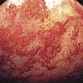
Figure 5.1 shows a plot of the surviving fraction of cells as measured by the number of colonies formed by the surviving cells relative to the control. If a cell forms a colony, as shown in the photographs in Fig. 5.2, it is assumed to have survived irradiation and to have maintained its reproductive ability. This type of procedure is called a clonogenic assay or a survival assay.
Figure 5.2 Comparison of petri dishes containing (a) unirradiated and (b) irradiated cells. The difference in the number of surviving colonies is apparent to the naked eye. Source: Nias (1998), figure 6.6.
Cell Survival Curves: Quantification
In order to quantitatively interpret the results of cell survival assays, it is important to define two quantities: the plating efficiency and the surviving fraction.
Plating Efficiency
The plating efficiency is simply the percentage of seeded cells that survive to form colonies under control conditions (i.e., no radiation or other modifying factors):
(5.1) 
Knowing the plating efficiency allows one to normalize out effects that lead to cell death but are not attributable to radiation. For example, assume the plating efficiency is found to be 50%. Then, in a later experiment using the same cells and the same incubation conditions, half of the cells irradiated with a 1 Gy dose of X-rays survive. In this particular case, the 1 Gy dose had no measureable effect (i.e., the cells died at the same rate, with or without X-ray irradiation).
Surviving Fraction
Once the plating efficiency is determined, then a meaningful determination of the surviving fraction can be made, that is, the fraction of cells that survive or die due to the radiation that one is testing:
(5.2) 
Another way to compute the surviving fraction (equivalent to the above) is
(5.3) 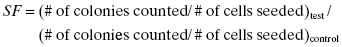
where “test” denotes the test condition (some radiation dose) and “control” denotes identical cells not treated with radiation.
Whichever equation is used, the important thing is to ensure that the surviving fraction is computed relative to the survival of a control population, in order to account for uninteresting factors that might influence cell survival (temperature, adequacy of the growth medium). This ensures that the effect of the radiation dose can be separated from the other factors.
Surviving Fraction versus Dose: The Cell Survival Curve
A plot of the surviving fraction of cells as a function of the radiation dose is called the cell survival curve. The survival curve is usually plotted on a log-linear graph (also referred to as a semilog plot) for reasons explained in detail later. The surviving fraction is plotted on the logarithmic axis (vertical) against dose, which is plotted on the linear axis (horizontal). Representative survival curves for high- linear energy transfer (LET) particles and low-LET radiation (X-rays) are shown in Fig. 5.3.
Figure 5.3 Representative cell survival curves for high-LET particles and low-LET X-rays. High-LET radiations produce curves that are steeper with little or no shoulder.
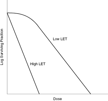
The shape of the high-LET curve is typical for mammalian cells irradiated by neutrons or alpha particles. The shape of the low-LET curve is typical for mammalian cells irradiated by X-rays, gamma rays, or beta particles. The low-LET curve is therefore the response that is expected when irradiating cells in conventional radiotherapy and diagnostic imaging. Survival curves for mammalian cells usually have a shoulder (curved section) in the lower-dose region, as shown in the low-LET curve. Models have been developed to account for survival curves with different shapes obtained under different conditions.
Modeling the Shape of the Survival Curve
There are three models used to mathematically describe cell survival curves: the single-target/single-hit model, the multitarget model (also known as the two-component model), and the linear–quadratic (LQ) model. Each model has its own advantages and disadvantages. The models are based on the idea of a “target” within the cell. The target is often viewed as a sensitive region on the DNA molecule that when hit by radiation may cause cell death.
The single-target/single-hit model has little practical application, but is useful in explaining the multitarget and LQ models. In the single-target/single-hit model, it is assumed that a cell has a single target that when hit causes the cell to die. In this case, the cell has no opportunity to repair the radiation damage. The single-target/single-hit model is inadequate to explain most cell survival data from mammalian cells, because it does not account for the shoulder portion of the curve at low doses.
The multitarget (two-component) and LQ models are both considered multiple-target models. Both models assume that each cell contains two or more targets that must be hit before the cell is killed. In order to be killed, the cell must accumulate enough hits in a short amount of time, such that the enzyme repair mechanisms are not capable of repairing all of the damage in between hits. However, after the first target is hit, the cell may have enough time to repair the damage before the next target is hit. In this case, the first hit is an example of sublethal damage. Sublethal damage occurs at a dose that is not sufficient to cause very much cell death. Thus, there are two dose regimes (low dose causing mostly sublethal damage, and high dose, causing lethal damage) that explain the shoulder (i.e., the change in slope) of the survival curve. Importantly, the multiple-target models provide a way to account for the presence of the shoulder region observed in mammalian cell survival curves. The multiple-target models fit the experimental data well, but still have limitations. Regardless of the underlying mechanisms, the major interest in survival curves data is in predicting radiation effects on humans.
Single-Target/Single-Hit Model
The simplest mathematical model to explain the radiation killing of cells is the single-target/single-hit model. In this model, a single hit on a single cellular target results in cell death. The curve from this model is shown in Fig. 5.4. The survival curve is exponential and can be fit by Equation 5.4:

Figure 5.4 Schematic representation of the single-target/single-hit survival curve. The survival curve is linear on a log-linear plot, with a slope of 1/D0.
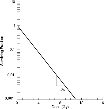
In this model, D is the dose delivered and D0 is a constant, defined as the dose that gives on average one hit per target. If there is one hit per cell on average, then statistically, some cells receive more than one hit, some receive exactly one hit, and some receive zero hits. In this case, Poisson statistics are used to describe the statistics of small numbers of random events—for example, 0, 1, 2. A dose D = D0 reduces the surviving number of cells to 37% of the initial population. Therefore, D0 is sometimes called D37. Note that D/D0 is the average number of hits per cell.
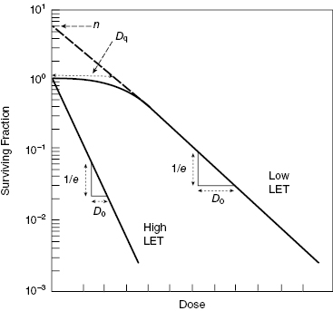
Taking the natural log (ln or loge) of both sides of the equation, one obtains
(5.5) 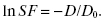
By plotting the quantity (ln SF) versus D, one obtains a straight line with slope –1/D0. Equivalently, one can plot the SF versus D on a log-linear scale, as shown in Fig. 5.4, and one will also obtain a straight line. The single-target/single-hit model can be used to describe data resulting from experiments involving viruses and bacteria, but is generally a poor model for describing mammalian cell survival.
Multitarget Model (also “Two-Component Model” or “Dq, D0, and n Model”)
Figure 5.5 shows typical survival curves for densely (high-LET) and sparsely ionizing (low-LET) radiations, along with definitions of the key parameters of the multitarget model, namely the parameters n, Dq, and D0.
Figure 5.5 Typical cell survival curves for high-LET (densely ionizing) and low-LET (sparsely ionizing) radiations. The parameter D0 characterizes the final slope of the curve. The parameter n or Dq characterizes the shoulder region of the low-LET curve.
The simplest equation for the multitarget model is
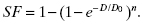
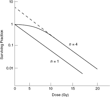
The parameter n was originally understood to be the number of targets in the cell. Notice that if n = 1, then Equation 5.6 reduces to Equation 5.4. In other words, the multitarget model reduces to the single-target/single-hit model for n = 1, as expected. This is illustrated in Fig. 5.6, which shows the results of Equation 5.6 evaluated for D0 = 2 Gy and n = 1 or 4. Notice that both curves have the same limiting slope at high dose, which turns out to be 1/D0, the same as in the single-target/single-hit model.
Thus, the multitarget model can be used to fit cell survival curves from either high-LET (no shoulder) or low-LET (shoulder) radiations by using different values of n (see Fig. 5.6). However, assuming that n is the number of critical targets leads to a logical inconsistency, because different values of n can be obtained for different types of radiation using the same cell type. If the cells are the same, but n changes with radiation type, n must depend on more than just the number of targets in the cell.
Figure 5.6 Multitarget model (Eq. 5.6) evaluated for D0 = 2 Gy and n = 1 or 4 shows the effect of different n values on the resulting survival curves.
The multitarget model may be further modified (to improve the shape of the curve in the low-dose region) by multiplying the multitarget term by a single-target term:
Equation 5.7 is the version of the multitarget model sometimes called the two-component model, because it has both a single-target and a multiple-target component. Multiplication by the single-target factor gives the curve a finite slope (of 1/D1) at D = 0. Equation 5.6 results in a curve with zero slope at D = 0.
The multitarget models do a reasonably good job of fitting real mammalian cell survival curve data, particularly in the high-dose region. Furthermore, the multitarget models give us a small number of parameters (D0, Dq, n), which are easy to determine graphically, as described later. By determining the parameters graphically, one avoids tedious calculations to obtain nonlinear least squares fits of Equation 5.6 or Equation 5.7. This was undoubtedly an advantage of these models before personal computers became ubiquitous.
Related posts:

Stay updated, free articles. Join our Telegram channel

Full access? Get Clinical Tree


