a Global Descriptor of Cardiac Motion from a Large Cohort of 1000+ Normal Subjects

Fig. 1.

The flowchart consists of motion tracking, spatial normalisation, descriptor learning and classification.

2 Methods

Prior to the learning of a motion descriptor, we first estimate motion from cine cardiac MR images. Since the heart of each subject lies at different locations and with different orientations, we perform spatial normalisation by registering and transporting all motion fields to a template space. The segmental motion trajectories are extracted and concatenated to form a high-dimensional feature vector. Dimensionality reduction is applied to the high-dimensional data leading to a global motion descriptor. Finally, we use the motion descriptor in exemplar classification tasks for gender classification and age prediction. Figure 1 illustrates the flowchart of the method and we will explain each step in the following.

2.1 Motion Tracking

In this work, we use cine MR for cardiac motion analysis. Other imaging modalities such as tagged MR or ultrasound (US) can also be used to capture the motion of the heart, which can provide different spatio-temporal resolution and image quality. The proposed motion descriptor is not confined to a specific imaging modality.

Motion tracking is performed for each subject using a 4D spatio-temporal B-spline image registration method with a sparseness regularisation term (TSFFD) [12]. The motion field estimate is represented by a displacement vector at each voxel and at each time frame t, which measures the displacement from the 0-th frame to the t-th frame. All the cine images in this work were acquired using the same imaging protocol, consisting of 20 time frames across a cardiac cycle with the 0-th frame representing the end-diastolic (ED) frame. Therefore, we do not perform temporal normalisation for the motion field.

2.2 Template Image and Spatial Normalisation

A template image is built by registering all the subject images at the ED frame and computing the average intensity image. In addition, the subject images are all segmented using a multi-atlas segmentation method [13]. The segmentation of the template image is then inferred by averaging all the subject segmentations. A template surface mesh is reconstructed from its segmentation and manually divided into 17 segments using the AHA model. The template and the segmental surface mesh are displayed at the top-right corner of Fig. 1.

The motion field estimate lies within the space of each subject. To enable inter-subject comparison and analysis, all the subject images are aligned to the template image by non-rigid B-spline image registration [14]. Using the transformation between the template space and subject space, we transport the motion field of each subject to the template space. Let $$x' = T(x)$$

denote the transformation from the template space to the subject space, where x and $$x'$$

are respectively the coordinates in the template space and in the subject space. By considering the spatial transformation as a change of coordinates, we have,

$\begin{aligned} d(x,t) = J_{T^{-1}}(x') d'(x',t) \end{aligned}$

(1)

where

denotes an infinitesimal displacement in the subject space, d denotes the corresponding infinitesimal displacement in the template space and $J_{T^{-1}}(x') \equiv \frac{dx}{dx'}$ denotes the Jacobian matrix of the inverse transformation.

2.3 Segmental Motion Trajectory

To characterise cardiac motion both spatially and temporally, we empirically define a high-dimensional feature vector using the segmental motion trajectory. S denotes the number of left ventricular segments. Since we use the AHA 17-segment model, $$S = 17$$

. T denotes the number of time frames, which is equal to 20 for our data set. d denotes the dimension of the displacement vector and $$d = 3$$

, which consists of radial, longitudinal and circumferential components. We compute the mean displacement for each segment at each time frame. The displacements across time for all the segments are concatenated to form the feature vector, which has the dimension of $S \times T \times d$ and contains information about the cardiac motion both spatially and temporally.

In principle, we can increase the spatial segments S so the feature vector describes more detailed motion at a higher spatial resolution. For example, we can compute the displacement for all the vertices of the myocardial mesh and concatenate them. However, we have found that it becomes computationally prohibitive to perform dimensionality reduction for vertex-wise motion data using techniques such as PCA. Also, since the cardiac motion is estimated using B-splines, displacements at neighbouring vertices are very similar and we may not need all the vertices to represent the motion data. Therefore, we adopt segment-wise motion data in this work.

2.4 Learning of a Motion Descriptor

Given the high-dimensional feature vector, we perform dimensionality reduction in order to find a descriptor which can characterise the motion with a low dimension. We compare two techniques, PCA and Isomap manifold learning [15]. The resulting low-dimensional coordinates are used as a motion descriptor.

PCA looks for a low-dimensional embedding of the data points that best preserves the variance. In the new coordinate system, the greatest variance of the data lies on the first coordinate, the second variance of the data on the second coordinate and so on. It is accomplished by eigen-decomposition of the data covariance matrix. In contrast to this, Isomap looks for a low-dimensional embedding that best preserves the geodesic distances between pairs of data points, i.e. the local data structure. It analyses the data structure as a graph, where each node denotes a data point and it is connected with K neighbours. The geodesic distances in the neighbourhood are preserved in the new coordinate system.

2.5 Application to Classification Tasks

To demonstrate the abundant information contained in the motion descriptor, we use the motion descriptor for two exemplar classification tasks, training SVM classifiers namely for gender classification and age prediction.

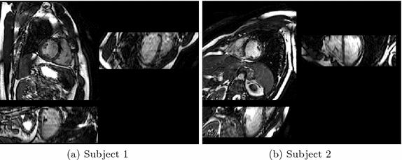
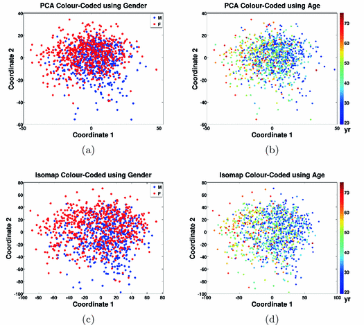
Fig. 2.

Two exemplar cardiac MR images. Three orthogonal views are shown for each subject.

Fig. 3.

Plot of the 1093 data points using the first two coordinates given by PCA (top row) or Isomap (bottom row). The data points are colour-coded using gender or age.

3 Experiments and Results

The data set used in this work consists of cardiac MR images of 1093 normal subjects (493 males, 600 females; age range 19–75 yr, mean 40.1 yr), which forms part of the UK 1000 Cardiac Phenomes project Cardiac MR was performed on a 1.5T Philips Achieva system (Best, Netherlands). The maximum gradient strength was 33 mT/m and the maximum slew rate 160 mT/m/ms. A 32 element cardiac phased-array coil was used for signal reception. Scout images were obtained and used to plan a single breath-hold 3D cine balanced steady-state free precession (b-SSFP) images in the left ventricular short axis (LVSA) plane from base to apex using the following parameters: repetition time msec/echo time msec, 3.0/1.5; flip angle, 50 $^{\circ }$ ; bandwidth, 1250 Hz/pixel; pixel size 2.0 $\times$ 2.0 mm; section thickness 2 mm overlapping; reconstructed voxel size, 1.25 $\times$ 1.25 $\times$ 2 mm; number of sections, 50–60; cardiac phases, 20; sensitivity encoding (SENSE) factor, 2.0 anterior-posterior and 2.0 right-left direction. Two exemplar images are displayed at Fig. 2.

Only gold members can continue reading. Log In or Register to continue