0.05 mm. And testing on data sets of 50 real images showed promising results.
Electronic supplementary material
The online version of this chapter (doi:10.1007/978-3-319-20309-6_15) contains supplementary material, which is available to authorized users.
Keywords
Rigid registration of 3D echocardiographyExtension of field of viewFarnebäck optic flowA. Danudibroto—Supported by Marie Curie Initial Training Network (USART-project, grant ID: PITN-GA-2012-317132).
M. Alessandrini—Supported by the Flemish Research Council (FWO), grant ID: 1263814N.
1 Introduction
3D echocardiography has brought added value to ultrasound imaging in clinical practice. In comparison to its 2D counterpart, 3D echo provides more anatomical information on the spatial relationship between structures. It assists in the diagnostic process and helps in training new echocardiographers. Its real time capability makes 3D echo a suitable imaging modality for intraoperative monitoring [11].
One of the inherent limitations of 3D echo is its dependence on the incidence angle [8]. Signal dropouts often occurs in the presence of strongly reflective structures. Transesophageal Echocardiography (TEE) and Intracardiac Echocardiography (ICE) probes that have a clear access to the heart during minimally invasive procedures have limited field of view due to their small aperture size.
There have been attempts to overcome these limitations using post-processing techniques, aiming at both improvement of image quality as well as extension of field of view. Such approaches are mainly focused on compounding information from several acquisitions. When combining image data from several acquisitions, they must be both registered and fused. Registration is performed to optimally transform the images into one common coordinate system while fusion combines the redundant data for optimal visual. Some studies focused more on the accuracy of the registration [2, 13, 14], while others at the improvement of image quality through fusion [1, 9, 16]. This paper focuses on the registration part.
Some studies utilize tracker information for registration [2, 16]. Either electromagnetic or optical trackers are commonly used. For electromagnetic tracking, there is a risk of disturbance in the electromagnetic field when ferro magnetic material is present. In the case of optical tracker, a clear line of sight from the optical marker to the sensor has to be kept.
Image based registration methods can be grouped into voxel based and feature based methods. Many available registration methods rely on optimization of a cost or similarity function that is computed directly from the voxel intensity values. Some of the known functions are: sum of absolute differences, sum of squared differences, normalized cross correlation (NCC) and mutual information [1, 12, 15]. Voxel based methods are to some extent dependent on pose initialization. Some works used tracker information for initial registration then refined it using a voxel based method [2, 16]. Other approaches also perform optimization but on extracted features from the image instead of directly on the intensity values. For example, Ni et al. [13] utilized 3D SIFT which is a scale invariant and robust gradient based feature descriptor to perform registration on 3D ultrasound of the liver to build panoramic volumes. Similarly, Schneider et al. [14] used features based on Laplacian-of-Gaussian filtering to register images of a porcine heart in a water tank while Grau & Noble [9] used monogenic signal analysis.
In this work, a new approach is proposed. The proposed registration is based on signal decomposition into a polynomial basis using the optical flow method by Farnebäck [5]. Farnebäck optic flow was chosen for its ability to handle potential uncertainty in the images. In contrast to the voxel based methods that optimize global cost function by applying a series of transformations, the Farnebäck method attracts the floating image to the optimum position and orientation that matched the reference image based on the analytical solution of the optic flow problem. This approach was taken to allow for robust and fast registration in images with very small frame-to-frame transformations as well as larger transformations.
2 Methodology
The general overview of the proposed registration method can be seen in Fig. 1.
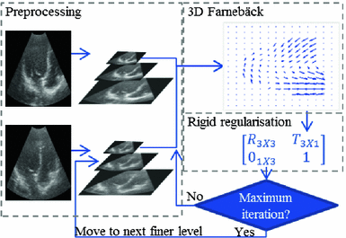
Fig. 1.
Overview of registration method
2.1 Preprocessing
Before registration, three preprocessing steps were performed. First, to eliminate influence from the background and shadow regions, a high intensity mask was applied. In ultrasound images, the shape of the sector is one of the dominant image structures. However, this structure does not provide useful information for registration.
To ensure that the algorithm is not directionally biased, the images were resliced so that the voxel dimension is isometric. Lastly, to reduce computation time and increase the range of detectable transformations, Gaussian pyramids were built for both reference and floating images using an adapted method of impyramid function in MATLAB for 3D matrices.
2.2 Polynomial Decomposition
The registration approach is based on the work of Farnebäck [5, 6]. Farnebäck utilized signal analysis using orientation tensors to compute disparity between a pair of images. It modeled the signal with polynomial basis functions weighted by an applicability function that determined the neighborhood’s importance in signal analysis. The image was decomposed locally by means of normalized convolution as explained in [5] and approximated by a polynomial as in (1). In the case of 3D images, the position vector  consists of
 ![$$[x, y, z]^T$$](/wp-content/uploads/2016/09/A339585_1_En_15_Chapter_IEq3.gif) . When expanded, it can be seen that the polynomial used 10 basis functions as seen in (2).
. When expanded, it can be seen that the polynomial used 10 basis functions as seen in (2).
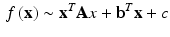
![$$\begin{aligned} \left[ 1, x, y, z, x^2, y^2, z^2, xy, xz, yz\right] \end{aligned}$$](/wp-content/uploads/2016/09/A339585_1_En_15_Chapter_Equ2.gif)
The choice of applicability function is crucial to appropriately express the image description by a set of polynomial coefficients. In this case it should decay as it moves away from the center voxel of interest, and be isotropic to avoid biases towards any direction in the neighborhood, hence a Gaussian function was chosen. Ideally, the  of the Gaussian applicability function would be comparable to the size of the feature of interest.
consists of . When expanded, it can be seen that the polynomial used 10 basis functions as seen in (2).(1)
(2)
of the Gaussian applicability function would be comparable to the size of the feature of interest.2.3 Rigid Transform Regularization
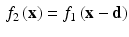
Based on the optic flow assumption, the floating image ( in (3)) is a transformed version of the reference image (
 in (3)). The disparity between a pair of images was computed using this assumption. Once expanded with the expression on (1), the disparity can be solved by equating the coefficients and can be expressed as (4). Note that the disparity is independent from the constant term c which means the local brightness should not affect the result. In ultrasound image analysis, this could be an advantage because the appearance of structures is incident angle dependent. Moreover the inherent signal uncertainty consideration allowed for focusing the optic flow computation only on the overlap region excluding the signal dropouts area. Although the speckle appearance might differ due to varying probe positions, the second order polynomial representation of the image limited the optic flow consideration to more dominant structures. Furthermore the Gaussian filtering in the preprocessing smoothed it out to an extent.
 Motion Estimation Using Ultrafast Ultrasound Imaging Tested in a Finite Element Model of Cardiac Mechanics
 Recognition in Cardiac CT Images
 Anisotropic Myocardial Stiffness from Magnetic Resonance Elastography: A Simulation Study
 and Biomechanics Inspired Integration of Shape and Speckle Tracking for Cardiac Deformation Analysis
 Stiffness Estimation: A Novel Cost Function for Unique Parameter Identification
 of the Electrocardiography Inverse Solution to the Torso Conductivity Uncertainties


in (3)) is a transformed version of the reference image ( in (3)). The disparity between a pair of images was computed using this assumption. Once expanded with the expression on (1), the disparity can be solved by equating the coefficients and can be expressed as (4). Note that the disparity is independent from the constant term c which means the local brightness should not affect the result. In ultrasound image analysis, this could be an advantage because the appearance of structures is incident angle dependent. Moreover the inherent signal uncertainty consideration allowed for focusing the optic flow computation only on the overlap region excluding the signal dropouts area. Although the speckle appearance might differ due to varying probe positions, the second order polynomial representation of the image limited the optic flow consideration to more dominant structures. Furthermore the Gaussian filtering in the preprocessing smoothed it out to an extent.Related posts:
Motion Estimation Using Ultrafast Ultrasound Imaging Tested in a Finite Element Model of Cardiac Mechanics
Anisotropic Myocardial Stiffness from Magnetic Resonance Elastography: A Simulation Study
Stay updated, free articles. Join our Telegram channel
Full access? Get Clinical Tree
