Fig. 1.
Top row: standard cardinal views (from left: axial, sagittal, coronal). Bottom row: non-cardinal (from left: four chamber (4C), short axis (SHA), two chamber (2C)).
2.2 Features
Group 1 – Statistical Image Texture Features: These include features calculated directly from the image (minimum value, maximum value, mean, range, standard deviation, median, central moment, square sum, average top quartile, average bottom quartile), and also those extracted from the co-occurrence matrices (entropy, energy, homogeneity). These features are calculated at different levels of granularity. Namely, we have included both the global feature calculated over the entire image, and also over image partitions that divide the image into 2  2, 3
2, 3  3, 5
3, 5  5, 7
5, 7  7 grids. The resulting features are concatenated to create a feature vector, per image.
2, 3 3, 5 5, 7 7 grids. The resulting features are concatenated to create a feature vector, per image.Group 2 – Curvelet Features: Curvelet features are proposed as a solution to overcome the limitations of wavelet as a multi-scale transform. We used the implementation reported in [9]. This curvelet methodology builds a multiscale pyramid in a Fourier-Mellin polar transform. Pyramid levels in the radial dimension consist of 1, 2, 4, and 8, and in the angular dimension the levels are 1, 2, 4, 8, 16, and 32 sections. Due to the large size of the feature vector, we only used the global granularity for this group of features.
Group 3 – Wavelet Features: This group consists of 120 texture features obtained by discrete wavelet transform at each granularity.
Group 4 – Edge Histogram Features: These are from a histogram of edge directions in the image in 64 bins resulting in 64 features, calculated per global, 2  2 and 3
  3 granularity levels.
2 and 3 3 granularity levels.Group 5 – Local Binary Pattern (LBP) Features: LBPs are calculated by dividing the image into cells, and comparing the center pixel with neighboring pixels in the window [10]. A histogram is built that characterizes how many times, over the cell, the center pixel is larger or smaller than the neighbors. In the implementation used here, the histogram is built on different scales (1, 1/2, 1/4 and 1/8 of the image), and a combined 59 dimensional histogram is produced. In this implementation, the LBP features are weighted by the inverse of the scale [9].
Group 6 (Proposed in this Work) – A Global Binary Pattern (GBP) of the Image: This proposed set of features relies on the pattern of high intensity components of the anatomy of the chest, including the ribs and vertebrae. The images are first pre-processed with histogram equalization to a range routinely utilized by radiologists to maximize the contrast in cardiac chambers and vessels. Then multi-level Otsu thresholding, with four levels, is applied [11]. Otsu thresholding calculates the optimal thresholds to minimize intra-level variance. The highest intensity level is then subjected to connected component clustering. The resulting connected components are then filtered based on the size of the area. An area size of 30 pixels is used in images of size 512 512. Samples of the resulting binary images are presented in Fig. 2. The binary image is then re-sized and down-sampled to obtain an
  matrix, where m is chosen by experimentation from values of
 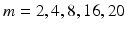 . In Fig. 2, examples of this matrix for
  are shown. The feature vector used for this method is the
  vector generated by concatenating the columns of this matrix.
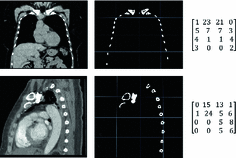
512. Samples of the resulting binary images are presented in Fig. 2. The binary image is then re-sized and down-sampled to obtain an matrix, where m is chosen by experimentation from values of . In Fig. 2, examples of this matrix for are shown. The feature vector used for this method is the vector generated by concatenating the columns of this matrix.Fig. 2.
Examples of converting a coronal (top row) and sagittal (bottom row) cardiac CT image to a set of 16 GBP features.
2.3 Classification
We used a support vector machine (SVM) classifier for each feature category. Given the large size of the feature vectors and the relatively small size of the dataset, we do not combine the six different categories of features into a single vector. Instead, we use individual SVMs and combine with voting. SVM training optimizes w and b to obtain the hyperplane  where
where  is the feature vector and
  is the kernel function, to maximize the distance between the hyperplane and the closest samples (support vectors) in the two classes. SVM is by definition a binary classifier. In the current work, we need to solve three and six-class classification problems. We used a one-versus-all approach to decide the label of each image for each feature group. In this approach, for an n class classification, we train n classifiers each separating one of the viewpoint types from the rest of images. Each test sample is classified by the n classifiers, and “class likelihood” is calculated as described below for each of the n classifiers. The label with the largest class likelihood obtained from its corresponding one-versus-all classifier is chosen as the viewpoint suggested by the feature group for the test sample. In order to calculate the class likelihood, we use the method described in [12]. Given the SVM hyperplane obtained in training, the class likelihood (
 ) for class c for test sample
  is computed using a sigmoid function of form:
where  and
and  are calculated using maximum likelihood estimation on the training data. We experimented with three different kernel functions. These were the linear kernel, radial basis function (RBF), and the polynomial kernel. There was no advantage in terms of accuracy when RBF or polynomial kernel were used. We report the results obtained using the linear kernel where
  .
.
where is the feature vector and is the kernel function, to maximize the distance between the hyperplane and the closest samples (support vectors) in the two classes. SVM is by definition a binary classifier. In the current work, we need to solve three and six-class classification problems. We used a one-versus-all approach to decide the label of each image for each feature group. In this approach, for an n class classification, we train n classifiers each separating one of the viewpoint types from the rest of images. Each test sample is classified by the n classifiers, and “class likelihood” is calculated as described below for each of the n classifiers. The label with the largest class likelihood obtained from its corresponding one-versus-all classifier is chosen as the viewpoint suggested by the feature group for the test sample. In order to calculate the class likelihood, we use the method described in [12]. Given the SVM hyperplane obtained in training, the class likelihood () for class c for test sample is computed using a sigmoid function of form:(1)
and are calculated using maximum likelihood estimation on the training data. We experimented with three different kernel functions. These were the linear kernel, radial basis function (RBF), and the polynomial kernel. There was no advantage in terms of accuracy when RBF or polynomial kernel were used. We report the results obtained using the linear kernel where .Voting: The resulting six classifiers return six potentially different viewpoints for each image. In order to determine the final image label and maximize the accuracy, we used a majority voting scheme where the class label is determined as the most frequently returned label among the six classifiers. The result is reported as “correct” only if at least three classifiers return the correct label. There was no tie (3 to 3) vote in our experiments. However, a potential tie can be decided based on the average class likelihoods.
Training and Testing Strategy: We used a leave-one-sample out strategy for training and testing. Each sample serves as the hold-out once. For each of the classification problems, all feature specific classifiers are trained using all but the hold-out sample and the hold-out is used as the test sample. This is repeated until all samples are tested. In the six-class problem, six one-versus-all classifiers are trained per feature type which adds up to 36 SVMs to be trained for each leave-one-out step. In the three-class problem, there are 18 SVMs to be trained. Note that in all of these training and testing experiments, a linear SVM with similar parameters is employed. The SVM slack variable is set to  .
.
.Related posts:
 Motion Estimation Using Ultrafast Ultrasound Imaging Tested in a Finite Element Model of Cardiac Mechanics
Stay updated, free articles. Join our Telegram channel

Full access? Get Clinical Tree


