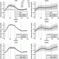
uncertainties in the fat conductivity does not alter the inverse solution, whereas adding  uncertainties in the lung conductivity affects the reconstructed heart potential by almost
  .
.
1 Introduction
The ECGI procedure helps medical doctors to target some triggers of cardiac arrhythmia and consequently plan a much more accurate surgical interventions [1]. The mathematical problem behind the ECGI solution is known to be ill posed [2]. Therefore, many regularization techniques have been used in order to solve the problem [3–7]. Thus, the obtained solution depends on the regularization method and parameters [8]. Furthermore, the inverse solution does not depend only on the regularization method but also to the physical parameters and the geometry of the patient. These dependencies have not been taken into account in most (if not all) of the studies. In particular, in most of the studies in the literature the torso is supposed to be a homogenous. Moreover, when the conductive heterogeneities are considered, they are fixed according to data obtained from textbooks. The problem is that these data are different from a paper to another [9–11]. Their variability is mainly due to the difference between the experiment environments and other factors related to the measurement tools. Only few works have been performed in order to study the effect of conductivities uncertainty in the propagation of the electrical potential in the torso [12–14]. In [13], authors use the stochastic finite elements method (SFEM) to evaluate the effect of lungs muscles and fat conductivities on the forward problem. In [14], authors used a principal component approach to predict the effect of conductivities variation on the body surface potential.
However, to the best of our knowledge, no work in the literature has treated the influence of conductivity uncertainties of the ECGI inverse solution. In this work, we propose to use an optimal control approach to solve the inverse problem and to compute the potential value on the heart, we use an energy functional [15]. with SPDE constraints as proposed in [13]. We are interested in assessing the effect of the variability of tissue conductivity on the solution of the ECGI problem. The resolution of optimal control will be made using an iterative procedure based on the conjugate gradient method and the numerical approximation will be performed using the SFEM.
2 Methods
2.1 Solving Stochastic Forward Problem of Electrocardiography
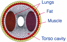
Following [13], we represent the stochastic characteristics of the forward solution of the Laplace equation by the generalized chaos polynomial. For the space domain we use simplified analytical 2D model representing a cross-section of the torso (see Fig. 1) in which the conductivities vary stochastically. Let us first denote by D the spatial domain and  the probability space. By supposing that the conductivity parameter depends on the space and on the stochastic variable
  the solution of the Laplace equation does also depend on space and the stochastic variable
  The stochastic forward problem of electrocardiography can be written as follows:
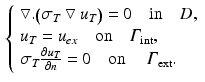
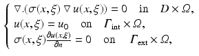
where,  and
and  are the epicardial and torso boundaries respectively,
  is the stochastic variable (it could also be a vector) and
  is the potential at the epicardial boundary.
the probability space. By supposing that the conductivity parameter depends on the space and on the stochastic variable the solution of the Laplace equation does also depend on space and the stochastic variable The stochastic forward problem of electrocardiography can be written as follows:(1)
and are the epicardial and torso boundaries respectively, is the stochastic variable (it could also be a vector) and is the potential at the epicardial boundary.2.2 Numerical Descretization of the Stochastic Forward Problem
We use the stochastic Galerkin (SG) method in order to solve Eq. (1). A stochastic process  of a parameter or a variable X is represented by weighted sum of orthogonal polynomials known as probability density functions PDFs
  More details about the different choices of PDFs could be found in [16]. In our case we use the Legendre polynomials which are more suitable for uniform probability density.
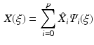 where
where  are the projections of the random process on the stochastic basis
  The mean value and the standard deviation of X over
  are then computed as follows
![$$\begin{aligned} \text {E} (X)=\int _{{\varOmega }}\sum ^{p}_{i=0}\hat{X}_{i}{\varPsi }_i(\xi )= \hat{X}_{0}, \quad \text {stdev} [X]= \big (\sum ^{p}_{i=1}\hat{X}_{i}^{2} \int _{{\varOmega }} {\varPsi }_{i}(\xi ) ^{2} \big )^{\frac{1}{2}} \end{aligned}$$](/wp-content/uploads/2016/09/A339585_1_En_54_Chapter_Equ13.gif) Since in our study we would like to evaluate the effect of the conductivity randomness of the different torso organs on the electrical potential. Both of
Since in our study we would like to evaluate the effect of the conductivity randomness of the different torso organs on the electrical potential. Both of  and u are now expressed in the Galerkin space as follows:
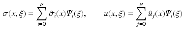 By substituting (2), (3) into the elliptic Eq. (1) and by projecting the result on the polynomial basis
  we obtain the following system: For
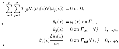
where ![$$T_{ijk}=E[{\varPsi }_i(\xi ),{\varPsi }_j(\xi ),{\varPsi }_k(\xi )].$$](/wp-content/uploads/2016/09/A339585_1_En_54_Chapter_IEq19.gif) By applying the standard finite elements variational formlation and Galerkin projections we obtain a linear system of size
By applying the standard finite elements variational formlation and Galerkin projections we obtain a linear system of size  where dof is the number of the degrees of freedom for the Laplace equation in the deterministic framework.
of a parameter or a variable X is represented by weighted sum of orthogonal polynomials known as probability density functions PDFs More details about the different choices of PDFs could be found in [16]. In our case we use the Legendre polynomials which are more suitable for uniform probability density. are the projections of the random process on the stochastic basis The mean value and the standard deviation of X over are then computed as follows and u are now expressed in the Galerkin space as follows: we obtain the following system: For (2)
By applying the standard finite elements variational formlation and Galerkin projections we obtain a linear system of size where dof is the number of the degrees of freedom for the Laplace equation in the deterministic framework.Fig. 1.
2D computational mesh of the torso geometry showing the different regions of the torso considered in this study (fat, muscle, lungs, torso cavity).
2.3 Stochastic Inverse Problem Problem
In this section we propose to build an optimal control problem taking into account the variability of the tissue conductivities in the torso. Let us first propose a gold standard solution representing the true electrical potential in the torso. Supposing that the true conductivity distribution in the torso is  at a given time the true electrical potential in the torso
  is governed by the Laplace equation, it depends on the extracellular potential at the epicardium
  as follows:
From the deterministic forward problem solution  we extract the electrical potential at the external boundary and we denote it by
  For the inverse problem formulation, we write a cost function that takes into account the uncertainties in the torso conductivities. We then use an energy cost function as used in [15, 17] constrained by the stochastic conductivity Laplace formulation as presented in the previous paragraph. We look for the current density and the value of the potential on the epicardial boundary
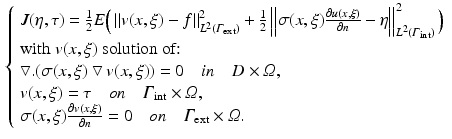
  minimizing the following cost function
In order to solve this minimization problem, we use a conjugate gradient method as used in [15] where the components of the gradient of the cost function are computed using an adjoint method. The gradient of the functional J is given by:
![$$\begin{aligned} \left\{ \begin{array}{ll} <\frac{\partial J(\eta ,\tau )}{\partial \eta }. \phi >= – E[\int _{{\varGamma }_{\text {int}}}(\sigma \frac{\partial v}{\partial n}-\eta )\phi d{\varGamma }_{\text {int}}]\quad \forall \, \phi \in L^{2}({\varGamma }_{\text {int}}),\\ <\frac{\partial J(\eta ,\tau )}{\partial \tau }. h>=E[\int _{{\varGamma }_{\text {int}}}\sigma \frac{\partial \lambda }{\partial n}h d{\varGamma }_{\text {int}}]\quad \forall \, h \in L^{2}({\varGamma }_{\text {int}}),\\ \text {with } \lambda \text { solution of:}\\ \nabla .(\sigma (x,\xi )\nabla \lambda (x,\xi ))=0 \quad \text { on } D\times {\varOmega }, \\ \lambda (x,\xi )=\sigma (x,\xi )\frac{\partial v(x,\xi )}{\partial n}-\eta \quad \text { on } {\varGamma }_{\text {int}}\times {\varOmega }, \\ \sigma (x,\xi )\frac{\partial \lambda (x,\xi )}{\partial n}=-(v-f) \quad \text { on } {\varGamma }_{\text {ext}}\times {\varOmega }. \end{array}\right. \end{aligned}$$” src=”/wp-content/uploads/2016/09/A339585_1_En_54_Chapter_Equ5.gif”></DIV></p>
<div class='tao-gold-member'>
<div>Only gold members can continue reading. <a href='/login'> Log In</a> or<a href='/register'> Register </a> to continue</div>
</div>
<p></p>
<div class=]()
 Motion Estimation Using Ultrafast Ultrasound Imaging Tested in a Finite Element Model of Cardiac Mechanics
 Recognition in Cardiac CT Images
 Anisotropic Myocardial Stiffness from Magnetic Resonance Elastography: A Simulation Study
 Feature Learning for Myocardial Segmentation of CP-BOLD MRI
 Biomechanical Modeling of Cardiac Amyloidosis – A Case Study
 Edge Map (PEM) for 3D Ultrasound Image Registration and Multi-atlas Left Ventricle Segmentation


at a given time the true electrical potential in the torso is governed by the Laplace equation, it depends on the extracellular potential at the epicardium as follows:(3)
we extract the electrical potential at the external boundary and we denote it by For the inverse problem formulation, we write a cost function that takes into account the uncertainties in the torso conductivities. We then use an energy cost function as used in [15, 17] constrained by the stochastic conductivity Laplace formulation as presented in the previous paragraph. We look for the current density and the value of the potential on the epicardial boundary minimizing the following cost function(4)
Related posts:
Motion Estimation Using Ultrafast Ultrasound Imaging Tested in a Finite Element Model of Cardiac Mechanics
Anisotropic Myocardial Stiffness from Magnetic Resonance Elastography: A Simulation Study
Biomechanical Modeling of Cardiac Amyloidosis – A Case Study
Stay updated, free articles. Join our Telegram channel
Full access? Get Clinical Tree
