Arterial Spin Labeling for Functional Neuroimaging
Thomas T. Liu
Since it inception over 20 years ago, functional magnetic resonance imaging (fMRI) has been primarily based on MR pulse sequences that utilize blood oxygenation level dependent (BOLD) contrast. Although BOLD fMRI offers both a high contrast-to-noise ratio and good spatial and temporal resolution, the interpretation of the BOLD signal as a reflection of neural activity can be complicated by its dependence on changes in cerebral blood flow (CBF), the cerebral rate of oxygen metabolism (CMRO2), and cerebral blood volume (CBV). Variations in any of these physiologic quantities because of age, disease, or the presence of vasoactive agents1,2,3 can confound the interpretation of changes in the BOLD signal across groups and conditions.
Perfusion fMRI based on arterial spin labeling (ASL) methods can provide quantitative measures of functional changes in CBF and offers a useful complement to BOLD fMRI. When using ASL for fMRI, we are interested in measuring the dynamic changes in CBF that occur over time in response to either external stimuli (e.g., a flashing checkerboard pattern) or as a reflection of intrinsic spontaneous brain activity (e.g., resting-state neural fluctuations). From these dynamic measures, we can make a map indicating where there are statistically significant changes in CBF, characterize the amplitude of these changes and their spatial distribution, examine the functional connectivity between brain regions, and also examine features of the dynamic response, such as rise and fall times. This chapter discusses the key issues that need to be considered when using ASL for fMRI studies: (a) choice of acquisition and processing methods; (b) temporal resolution; (c) spatial coverage and spatial resolution, (d) signal-to-noise ratio; (e) quantitative accuracy; and (f) ability to yield additional contrasts of interests. In reviewing these issues, BOLD fMRI will be used as a reference point. Additional reviews of the use of arterial spin labeling for fMRI can be found elsewhere.4,5,6
Acquisition
Most ASL methods measure CBF by taking the difference of two sets of images: tag images, in which the magnetization of arterial blood is inverted or saturated, and control images, in which the magnetization of arterial blood is fully relaxed. The difference between the control and tag images yields an image that is proportional to the blood that has been delivered. There are a variety of ASL methods that have been developed, and these methods can be divided into three main classes: (a) pulsed ASL (PASL) in which short radiofrequency (RF) pulses are used to tag the blood over an extended spatial region that is proximal to the imaging region of interest; (b) continuous ASL (CASL) in which a long (on the order of several seconds) RF waveform or train of pulses is used in conjunction with gradient fields to tag flowing blood spins as they traverse an irradiated plane (this class also includes pseudo-continuous ASL [pCASL]); and (c) velocity-selective ASL (VS-ASL) in which an RF pulse train is applied that selectively saturates flowing spins with no spatial selectivity. Greater detail on the various approaches can be found in Chapters 15 through 22 in this book. The relative advantages and disadvantages of these methods for perfusion fMRI will be discussed in the sections below.
Aside from the use of different pulse sequence and acquisition parameters, the mechanics of an ASL fMRI experiment are similar to those of a BOLD fMRI experiment, with data being acquired as the subject is either performing a task (i.e., task state) or lying quietly (i.e., control or rest state) in the scanner. With real-time processing and analysis of the data,7 there is also the opportunity for fMRI-guided biofeedback in which the subject attempts to modify his or her brain activity in response to an fMRI indicator of the brain response.
Processing
In most ASL fMRI experiments, control and tag images are acquired in an interleaved fashion, as shown in Figure 76.1. A perfusion time series is then formed from the running subtraction of the control and tag images. An example of this process is shown in Figure 76.1, where the perfusion images are formed from the difference between each control image and the average of the two surrounding tag images or from the difference between the average of two surrounding control images and a tag image. The type of differencing shown in Figure 76.1 is referred to as surround subtraction, and it represents one specific approach to the filtered subtraction of control and tag images. Given an interleaved acquisition of the form (e.g., Tag[0], Control[0], Tag[1], Control[1], …), surround subtraction over the image acquisition time series produces the perfusion weighted time series: (Control[0] − (Tag[0] + Tag[1])/2], (Control[0] + Control[1])/2 − Tag[1], …). Other common approaches are pairwise subtraction and sinc subtraction. Pairwise subtraction would generate a perfusion weighted time series of the form: (Control[0] − Tag[0], Control[0] − Tag[1], Control[1] − Tag[1], …). The sinc subtraction method can be considered an extension of the surround subtraction method that uses a greater number of tag and control
images to form the perfusion estimate at each time point, where the coefficients used to multiply the tag and control images are determined by the values of a mathematical function called the sinc function.
images to form the perfusion estimate at each time point, where the coefficients used to multiply the tag and control images are determined by the values of a mathematical function called the sinc function.
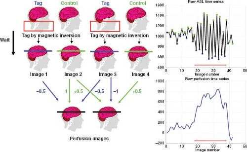 FIGURE 76.1. Formation of a perfusion time series from the “surround subtraction” of control and tag images. The red box indicates the labeling slab. An example time series of control (green) and tag (blue) signals is shown in the upper right-hand plot. The red bars indicate the time of stimulus. The perfusion time series created by “surround subtraction” is shown in the lower right-hand plot. The red bars indicate the time of stimulus. Here, the first time point is generated by taking the average of images 1 and 3 (blue arrows) and subtracting it from image 2 (green arrow). Similarly, the second time point is generated by averaging images 2 and 4 (green arrows) and subtracting image 3 (blue arrow) from this average. |
A general analytic model has been developed to compare the performance of these three methods of subtraction,8 which all share the property that they can be modeled as the modulation of the control and tag images (e.g., multiply all control images by +1 and all tag images by −1) followed by convolution with a low-pass filter. One can also high-pass filter the data before modulating, as proposed by Chuang et al.9 It can be shown that this alternate process is mathematically equivalent to the process of modulation followed by low-pass filtering.
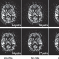
For fMRI experiments with block designs in which the stimuli are presented in long blocks (typically 20 to 40 seconds) interleaved with long blocks of a control state, surround and sinc subtraction tend to provide the best performance.10 In contrast, for randomized event-related designs in which the stimuli are presented in a rapid fashion with the intervals between stimuli, pair-wise subtraction can provide better performance (e.g., less filtering of the hemodynamic response function). Figure 76.2 shows examples of block and randomized event-related
designs. For the randomized event-related design, example response estimates obtained with the different subtraction methods are shown in Figure 76.3. All filtered subtraction approaches lead to inevitable broadening of the hemodynamic response function.8 Unfiltered approaches based on general linear models (GLM) of the ASL experiment can be used to eliminate this broadening11 and can lead to improvements in the ability to detect the presence of an activation or estimate the parameters of the response.12,13 Bayesian approaches to the analysis of ASL data also show promise for increasing the sensitivity of ASL measures.14
designs. For the randomized event-related design, example response estimates obtained with the different subtraction methods are shown in Figure 76.3. All filtered subtraction approaches lead to inevitable broadening of the hemodynamic response function.8 Unfiltered approaches based on general linear models (GLM) of the ASL experiment can be used to eliminate this broadening11 and can lead to improvements in the ability to detect the presence of an activation or estimate the parameters of the response.12,13 Bayesian approaches to the analysis of ASL data also show promise for increasing the sensitivity of ASL measures.14
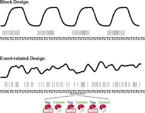 FIGURE 76.2. In an experiment that uses a block design, the stimuli (represented by the narrow vertical lines) are grouped together into blocks. The resulting cerebral blood flow (CBF) response is shown by the smooth curve with four cycles. In an experiment with a randomized event-related design, the stimuli are presented in a random fashion, and the resulting CBF response reflects this randomness. As shown at the bottom of the figure, Tag (T) and control (C) images are acquired in an interleaved fashion throughout the course of each experiment. |
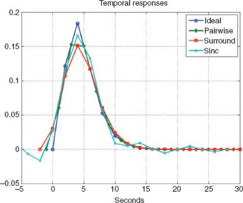 FIGURE 76.3. Cerebral blood flow response estimates obtained using a randomized event-related design with pairwise subtraction (green), surround subtraction (red), and sinc subtraction (cyan). For comparison, the ideal response is shown in blue. Additional details can be found in Liu and Wong.8 |
As with BOLD fMRI experiments, cardiac and respiratory fluctuations are a major source of noise in ASL experiments, especially at higher field strengths. Because the inherent signal-to-noise ratio (SNR) of ASL fMRI methods can be roughly one to two orders of magnitude lower than that of BOLD fMRI,10,15,16 the need for methods to reduce physiologic noise is especially pronounced. Retrospective image-based correction methods have been shown to significantly reduce physiologic
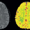
noise in ASL data.17,18 One approach requires the acquisition of external measures of cardiac and respiratory activity (e.g., with a pulse oximeter and respiratory effort transducer) and uses these measures to remove the associated physiologic noise components.18 In another approach, the physiologic noise components are estimated from the image data themselves, without the need for external measures.17 This latter approach takes advantage of the fact that signal fluctuations in the cerebral spinal fluid and white matter can provide estimates of the physiological noise components. Examples of the application of the different approaches are shown in Figure 76.4.
noise in ASL data.17,18 One approach requires the acquisition of external measures of cardiac and respiratory activity (e.g., with a pulse oximeter and respiratory effort transducer) and uses these measures to remove the associated physiologic noise components.18 In another approach, the physiologic noise components are estimated from the image data themselves, without the need for external measures.17 This latter approach takes advantage of the fact that signal fluctuations in the cerebral spinal fluid and white matter can provide estimates of the physiological noise components. Examples of the application of the different approaches are shown in Figure 76.4.
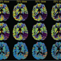
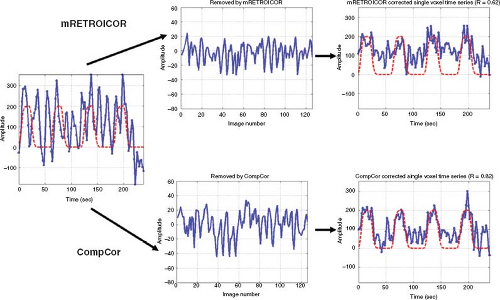 FIGURE 76.4. A noisy perfusion time series is shown on the left-hand side. The dashed red line indicates the model function representing the stimulus. Application of either model-based (e.g., using external measures of cardiac and respiratory activity) physiologic noise reduction (mRetroicor) or component-based noise reduction (CompCor) significantly increases the correlation between the perfusion time series and the model function, as shown by the greater degree of similarity between the time series and the model functions in the right-hand column. The noise time series that are removed by the processing methods are shown in the middle column. |
Temporal Resolution
The temporal resolution of perfusion fMRI is inherently poorer than BOLD fMRI because of the necessity to form tag and control images and to allow time for blood to be delivered from the tagging region to the imaging slice. In a typical PASL experiment, a repetition time (TR) of 2 seconds or more is used, so that one tag and control image pair is acquired every 4 seconds. For CASL, the TR is typically longer (on the order of 4 seconds) than for PASL, because of the longer time required for the CASL tagging process. With these time scales and the use of either CASL or PASL, it is generally reasonable to assume that, during the time interval between tags, the blood in the tagging region is refreshed with fully relaxed blood delivered by the systemic circulation. By comparison, the temporal resolution of BOLD fMRI is typically 1 to 2 seconds and can be as low as 100 milliseconds with more recently developed methods.19,20
Methods for improving temporal resolution include turbo-ASL21 and single-shot ASL.22 Turbo-ASL shortens the imaging time by placing the image acquisition at a short delay (typically 100 milliseconds) following the control to acquire the preceding tag signal and vice versa. In single-shot ASL, background suppression is used to suppress static tissue, thus eliminating the need for a control image. Although turbo-ASL and single-shot ASL can improve temporal resolution, the quantitation of the resultant ASL signals is more complicated than for the more standard methods.23 As a result, maps obtained using these approaches will be sensitive to changes in both CBF and transit delays (described in more detail below) and cannot be easily interpreted as a quantitative reflection of functional changes in perfusion. However, they may be useful for applications in which an investigator simply wants to know which areas of the brain exhibit perfusion-related dynamic changes in the MR signal.
Insensitivity to Low-Frequency Drifts
The lower temporal resolution of ASL is often considered a disadvantage because the reduced number of time points reduces the potential statistical degrees of freedom as compared with BOLD, where the degrees of freedom refer to the number of independent samples acquired in an experiment. In general, the ability to detect functional activity (i.e., probability of detection) at a specified significance level (i.e., probability of false alarm) increases as the degrees of freedom increase. However, ASL can provide an advantage in experiments where the signals of interest vary slowly with time. Low-frequency drifts are present in most BOLD fMRI time series data and tend to reduce the degrees of freedom and hence the statistical power of BOLD experiments. These drifts can be caused by systematic changes (e.g., heating of the permanent shims and the radiofrequency body coil because of aggressive switching of the gradients) in the MRI hardware and by slow variations in subject physiology. ASL can deal effectively with low-frequency confounds because most ASL fMRI experiments involve the acquisition of control and tag images in an interleaved fashion (i.e., they have an internal reference point). As described previously, a perfusion time series is then formed from the running subtraction of the control and tag images.8 This subtraction process greatly attenuates the low-frequency drifts that are unrelated to functional activity and can make ASL more sensitive than BOLD for experimental paradigms with long periods (i.e., long blocks) where a slow time course of functional activity is anticipated, such as the response to an administered drug.10 For example, one study has shown that the sensitivity of ASL is greater than that of BOLD when the alternating period between task and control is greater than a few minutes and also demonstrated that patterns of activation were detectable when comparing resting images on one day with activation images on the next day, a comparison that would not be possible with BOLD imaging.24
In a study assessing the effects of psychological stress on CBF, the insensitivity of ASL to low-frequency drifts enabled the investigators to demonstrate an increase in CBF that persisted for at least 8 minutes after the completion of a stressful task.25 Several recent studies have used ASL to look at slow changes in CBF associated with the administration of pharmacologic agents,26,27 sexual arousal,28 and the inducement of itching.29 Because ASL provides quantitative measures of CBF, it can also be used to measure changes that occur over several days or more, such as a change in CBF because of disease progression.
Spatial Coverage
At present, most ASL fMRI studies use two-dimensional multislice acquisition methods in which the data are acquired on a slice-by-slice basis. For CASL and PASL methods, the slices are typically acquired in an inferior-to-superior manner, so that slices that are further from the tagging region are acquired at later times. The number of slices that can be acquired depends on the (a) acquisition time for each slice, (b) the time (repetition time minus inversion time [TI]) that is available for slice acquisition, (c) the minimum TI that addresses transit delay issues (see below) and minimizes arterial contamination, and (d) the need to acquire slices before the difference signal, ΔM, has decayed away because of the longitudinal relaxation of blood. Because of these considerations, ASL fMRI studies typically acquire a smaller number of slices (e.g., 5 to 25 slices) than whole-brain BOLD studies (e.g., 30 to 40 slices), with thicker slices (e.g., 5 to 8 mm) than would be used in a BOLD study (e.g., 2 to 4 mm).
With advances in MRI methods, there is an increasing use of ASL fMRI studies with three-dimensional acquisitions that can offer whole-brain coverage, simultaneous acquisition of all slices, and greater SNR as compared with two-dimensional acquisitions.30,31,32 With the simultaneous acquisition of slices in a three-dimensional acquisition, the longitudinal relaxation of the tagged spins is the same across slices, leading to a greater consistency in SNR as compared with two-dimensional acquisitions, where the superior slices are acquired at a longer inversion time (with greater relaxation of the tagged spins) and can exhibit lower SNR as compared with the inferior slices.
Three-dimensional acquisitions with refocusing pulse trains can reduce susceptibility related artifacts, such as the severe signal dropouts that occur in the orbitofrontal cortex. In one study, ASL perfusion was shown to be less sensitive to susceptibility effects associated with overt speech than was the BOLD response.33 Three-dimensional acquisitions with low flip angle readouts have also been shown to be effective for perfusion mapping.34,35 There is typically a greater degree of through-plane blurring associated with three-dimensional acquisitions as compared with two-dimensional methods, but these effects can be partly addressed through the use of variable flip angles in the echo train or robust multishot acquisitions.35,36 The application of sparse MRI methods, such as compressed sensing, may also enable the faster acquisition of three-dimensional data with a reduction in blurring.37 Three-dimensional methods are also well suited to the use of background suppression methods for noise reduction (discussed further in the next section) because there is a specified point in time where all of the slices in a volume are excited, as compared with the sequential excitation times associated with two-dimensional acquisitions. The application of a three-dimensional acquisition with background suppression has been shown to improve the temporal SNR (i.e., signal-to-fluctuation noise ratio [SFNR]) and increase the statistical power of functional ASL scans.38 Some drawbacks of three-dimensional methods are (a) existing methods are not well suited for the simultaneous measurements of CBF and BOLD, which currently employs two-dimensional methods (see section below on CBF and BOLD estimates) and (b) when used with background suppression, estimates of CBF may be biased low.
Signal-to-Noise and Contrast-to-Noise Ratios
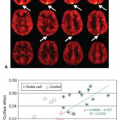
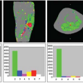
The SNR of ASL methods is inherently low because the inflowing blood magnetization typically comprises only about 1% of the overall tissue magnetization. Of the three major classes of ASL methods, CASL has the highest SNR, followed by PASL and VS-ASL.39,40,41 The low SNR combined with the poor temporal resolution of ASL results in a lower contrast-to-noise ratio (CNR) for ASL fMRI experiments as compared with BOLD. Figure 76.5 shows examples of CBF and BOLD maps showing the functional activation in response to a visual stimulus, with higher CNR values for the BOLD activation (as indicated by the greater proportion of red colors).
Related posts:
 Dose Considerations in CT Perfusion
 Confounding Effects in Arterial Spin Labeling
 Arterial Spin Labeling Acquisition Protocols
 Pediatric Stroke and Congenital Disease
 Clinical Applications of Dynamic Contrast-Enhanced Magnetic Resonance Imaging in Musculoskeletal Tumors
 Perfusion and Dynamic Contrast-Enhanced Imaging in White Matter Disease
Stay updated, free articles. Join our Telegram channel

Full access? Get Clinical Tree


