Confounding Effects in Arterial Spin Labeling

Danny J.J. Wang

María A. Fernández-Seara

Hanzhang Lu

Introduction

Perfusion imaging methods generally can be divided into three categories depending on the transport properties of the tracer: (a) microspheres that are deposited in the microvasculature, (b) intravascular or blood pool tracers that normally do not cross the blood–brain barrier (BBB), and (c) diffusible tracers that relatively freely diffuse into the tissue. Intravascular or blood pool tracers, such as gadolinium chelate for dynamic susceptibility contrast (DSC) magnetic resonance imaging (MRI) and iodinated contrast for computed tomography perfusion (CTP) imaging, are the most commonly used methods for measuring cerebral blood flow (CBF) in clinical settings. In DSC MRI or CTP, a bolus of contrast agent is injected intravenously and the response in the form of a transient decrease or increase in signal is monitored. With an independent measurement of the arterial input function (AIF), cerebral blood volume (CBV) and cerebral blood flow (CBF) can be determined using classical tracer kinetics, also allowing estimation of mean transit time (MTT) using the central volume principle.¹^,²^,³ More details about DSC MRI perfusion imaging can be found elsewhere in this book (see Chapters 11 to 14 and 24 to 28).

Arterial spin-labeled (ASL) perfusion MRI is a completely noninvasive method to measure CBF by utilizing magnetically labeled arterial blood water as an endogenous tracer. ASL belongs to the category of diffusible tracers, along with ¹⁵O-water and butanol positron emission tomography (PET), that theoretically are able to measure the “true” parenchymal perfusion. Compared to existing MRI, CT, and PET approaches that use external contrast agents or tracers, ASL has several advantages for absolute perfusion quantification. First, the AIF in ASL is explicitly defined by spatiotemporal parameters of labeling radiofrequency (RF) pulses; therefore, no arterial blood sampling as in PET or identification of arterial regions of interest (ROIs) as in DSC MRI and CTP are required, which are often sources of error in the existing methods. In addition, because ASL labels arterial blood proximal to the organ of interest, the dispersion of AIF should be much less, if not none, compared to an intravenously injected bolus. Second, because the tracer half-life determined by the T₁ of blood is relatively short in ASL (on the order of 1 to 2 seconds)—plus most labeled blood water diffuses into the tissue space—there is normally negligible venous outflow of the label in an ASL experiment. This property renders ASL analogous to a microsphere tracer method, leading to simplified models for perfusion quantification with reasonable accuracy. Last, estimation of CBF becomes highly complicated and challenging with a leaky BBB using existing DSC MRI and CTP methods relying on intravascular or blood pool tracers. (That said, the kinetics of tracer extravasation can be leveraged to interrogate BBB permeability as another diagnostic parameter.) ASL techniques, on the other hand, are much less sensitive to changes in BBB permeability given the small size of water molecules.

Given these potential advantages of ASL, there remain considerable concerns in the neuroimaging community whether ASL is able to provide accurate and reliable CBF measurements. One major challenge is the small fractional signal of the labeled blood (relative to the remaining tissue signal) considering that arterial blood volume is only 1% to 2% of total tissue volume in the brain. This small labeled signal further relaxes during its transit from the tagging region to the imaging slices, causing a relatively low signal-to-noise ratio (SNR) and arterial transit effects, that is focal signal trapped intravascularly yet to reach capillaries and tissue by the time of image acquisition. Because ASL relies on subtraction of label and control images, any imperfection between label and control acquisitions (besides spin labeling), such as unbalanced magnetization transfer (MT) effects, residual tissue signal from slice profile effects of the labeling pulses, and subject movements, can easily contaminate the perfusion signal. In addition, the generic ASL perfusion model often assumes constant parameters for the labeling efficiency, blood, and tissue T₁ while ignoring T₂/T₂^* relaxation and venous outflow. Some of these assumptions may be violated in clinical populations and different age groups. The purpose of this chapter is therefore to discuss potential confounding factors in ASL perfusion quantification, and further to propose calibration approaches to effectively address these issues.

Arterial Transit Effects

Arterial transit artifacts, manifested as focal intravascular signals in ASL images, are a major confounding factor for perfusion quantification. These artifacts result from an intravascular label that has not reached capillaries and tissue by the time image acquisition is carried out. For example, the arterial transit time (ATT) for the labeled blood to flow from the tagging region to the capillary/tissue can be
substantially elongated in patients with cerebrovascular diseases because of steno-occlusive abnormalities or collateral circulation.⁴ The general strategy to minimize the confounding effect of ATT is to apply a postlabeling delay time (PLD) that is longer than the ATT to allow the label sufficient time to flow into capillaries and tissue. In reality, the choice of the optimal PLD in clinical ASL applications is often an empirical decision by the investigator as the tradeoff between minimizing arterial transit artifacts and preserving the SNR, because the longer one waits the more label dies off owing to T₁ recovery.⁵ Such decision making may be difficult given the variability of ATT in clinical populations.⁶ When the PLD is not long enough, the ASL measurement is biased toward arteries and arterioles and tissue perfusion is underestimated. Although a long PLD can be applied, it reduces the SNR. In acute stroke, the prolonged ATT can be a major confounder for ASL-based CBF quantification (Fig. 18.1).

FIGURE 18.1. Comparisons of arterial spin-labeled (ASL) and dynamic susceptibility contrast (DSC) perfusion magnetic resonance imaging (MRI) in a series of four representative patients with acute ischemic stroke acquired within 24 hours of symptom onset. Fluid-attenuated inversion recovery (FLAIR) and diffusion-weighted imaging (DWI) are also shown. CBF, cerebral blood flow; CBV, cerebral blood volume; MTT, mean transit time. (Used with permission from Wang DJ, Alger JR, Qiao JX, et al. The value of arterial spin-labeled perfusion imaging in acute ischemic stroke–comparison with dynamic susceptibility contrast enhanced MRI. Stroke. 2012;43:1018–1024.)

Figure 18.1 shows side-by-side comparisons of ASL and DSC perfusion MRI in a series of four representative patients with acute ischemic stroke (AIS), all acquired within 24 hours of symptom onset.⁷ ASL was performed using pseudocontinuous ASL (pCASL) for spin labeling, three-dimensional (3D) background-suppressed (BS) GRASE (a hybrid of gradient and spin echo) as readout, and an intermediate PLD of 2 seconds. As can be clearly seen, hypoperfusion lesions in ASL CBF maps match best with prolonged time to the maximum of tissue residual function (Tmax) and MTT in DSC maps. ASL CBF is also consistent with DSC CBF calculated using standard singular value decomposition. This result suggests that hypoperfusion detected in ASL CBF maps may reflect both prolonged transit time and perfusion reductions in AIS and is therefore somewhat equivocal. Hence, although clinically ASL is valuable with similar information as DSC Tmax and MTT, its quantification of CBF with prolonged ATT remains a concern.

FIGURE 18.2. Cerebral blood flow maps of a moyamoya patient acquired using GRASE (a hybrid of gradient and spin echo) pseudocontinuous arterial spin labeling (pCASL) at four postlabeling delay times (PLDs; 800, 1400, 2000, and 2600 msec). Delayed arrival of the labeled blood in the right middle cerebral artery territory can be clearly seen (arrows).

Figure 18.2 shows CBF maps of a moyamoya patient that were acquired using GRASE pCASL at four PLDs (800, 1400, 2000, and 2600 msec). Delayed arrival of the labeled blood in the right middle cerebral artery (MCA) territory can be clearly seen. Even with the longest PLD
of 2600 msec, residual vascular signals (arrows) are present, suggesting that accurate perfusion quantification should be performed with PLD greater than 2600 msec.

Lately, there have been several new developments in the field of ASL that may provide potential solutions to address prolonged arterial transit effects. One approach is to map the ATT in vivo because transit time per se is a clinically meaningful physiologic parameter. Wang et al.⁸ have introduced such a technique termed flow-encoding arterial spin tagging (FEAST) that utilizes two ASL scans: one with and one without flow spoiling bipolar gradients, corresponding to the label that has exchanged into tissue and the total labeled blood signal, respectively. The ratios of both scans provide an estimate of ATT.⁸ For instance, delayed arrival of arterial bolus will leave a larger portion of the labeled blood in the vasculature by the time of image acquisition. This will lead to a reduced ratio of ASL signals in the tissue versus the total ASL signal in the affected vascular territory compared to control regions with normal ATT. An alternative approach is to simultaneously fit ATT and perfusion through continuous sampling of the dynamic inflow of the label, often using the Look-Locker (LL) approach.⁹^,¹⁰^,¹¹ Flow-spoiling gradients are commonly applied in LL and other image acquisitions for ATT measurement to specify the vascular compartment into which the labeled blood flows. Stronger gradients are able to spoil slower-flowing blood signals (in a way similar to diffusion imaging), thereby effectively targeting smaller vascular compartments. Figure 18.3 shows a comparison of ATT maps acquired using FEAST and LL-pCASL in a patient with left MCA blockage.¹² ASL CBF maps show prolonged arterial transit effects along with reduced tissue perfusion in the left MCA territory. Both FEAST and LL-pCASL show prolonged ATT in the corresponding area. In vivo measurement of ATT may be used as a prescan to determine the optimal PLD to be used for ASL studies. Alternatively, the measured ATT can be included in the CBF quantification model to improve its accuracy, assuming that the PLD is long enough to allow the labeled bolus to reach the brain region of interest.

FIGURE 18.3. Comparison of transit time maps acquired using flow-encoding arterial spin tagging (FEAST) and Look-Locker pseudocontinuous arterial spin labeling (LL-pCASL) in a patient with left middle carotid artery (MCA) blockage. CBF, cerebral blood flow. (Used with permission from Chen Y, Wang DJ, Detre JA. Comparison of arterial transit times estimated using arterial spin labeling. Magma. 2012;25:135–144.)

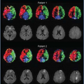
FIGURE 18.4. Comparison of cerebral blood flow (CBF) maps acquired using pseudocontinuous arterial spin labeling (pCASL) background-suppressed (BS) GRASE (a hybrid of gradient and spin echo) at a single postlabeling delay time (PLD) of 2 seconds and CBF, cerebral blood volume (CBV), and arterial transit time (ATT) maps acquired using multidelay pCASL BS GRASE with four PLDs at 1.5, 2, 2.5, and 3 seconds. Dynamic susceptibility contrast (DSC) CBF, CBV, and maximum of tissue residual function (Tmax)/mean transit time (MTT) maps are shown for comparison. FLAIR, fluid-attenuated inversion recovery; DWI, diffusion-weighted imaging;

More recently, largely owing to the development of fast 3D acquisitions, such as GRASE and SPIRAL, in conjunction with background suppression techniques, reliable ASL perfusion images at a single PLD can be acquired on the order of a few tens of seconds to 1 minute.¹³^,¹⁴ This fast imaging capability allows ASL scans at multiple PLDs to be performed within a few minutes for concurrent estimation of ATT, CBF, and arterial CBV through the central volume principle. An example of such a multidelay pCASL GRASE approach is shown in Figure 18.4. In the AIS case, CBF increases in hypoperfusion lesions using the multidelay protocol compared to that of a single PLD of 2s. The measured ATT is prolonged in hypoperfused regions, well matching DSC MTT and Tmax maps. Although the estimation of ATT and CBF may not be accurate for a severely prolonged transit time (>3 seconds), because of the T₁-based label decay, such a multidelay multiparametric ASL approach may significantly improve the accuracy and may expand the hemodynamic information offered by ASL in clinical settings.

Labeling Efficiency

CBF contrast in ASL is achieved by the inversion of arterial water magnetization in the labeled scan while keeping magnetization undisturbed in the control scan. Thus,
the degree to which these can be achieved in practice compared to theoretical maximum is usually referred to as the labeling efficiency.

FIGURE 18.5. Illustration of labeling pulse profile in relationship to imaging slices and labeling slab. Note that, if the gap between the imaging slices and labeling slab is insufficient, the imaging slices will be located in the transition zone, in which direct saturation by the labeling pulse is considerable and the cerebral blood flow is overestimated.

Confounding Factors in Pulsed Arterial Spin Labeling

Because PASL uses short RF pulses, the problem of labeling efficacy is essentially an RF pulse problem. This is not new to the MR community and has been extensively studied and optimized previously.¹⁵^,¹⁶^,¹⁷ A desired labeling RF pulse in PASL should have a flat inversion profile in the pass bands in the frequency domain, with a sharp transition between them.¹⁶ A large RF bandwidth is preferred because this allows the use of a large field gradient, reducing sensitivity to field inhomogeneity or tissue susceptibility differences. Whenever possible, an adiabatic RF pulse is used.¹⁸^,¹⁹^,²⁰ For implementations where adiabatic inversion is not feasible, such as the transfer-insensitive labeling technique (TILT), specially optimized RF pulses are often used.²¹ Simulations have demonstrated that typical PASL pulses can provide a labeling efficiency of 98%.²² The slight imperfection is due to the T₂ relaxation process during the period the RF is played out, which is around 10 to 20 msec. Because of the short RF pulse duration, the efficiency is relatively insensitive to flow velocity. It was found that, within a blood flow velocity range of 0 to 100 msec/second, the efficiency varies by less than 1%.²²

Because the RF slice profile is not exactly a step function (i.e., there is always a translational zone; Fig. 18.5), a gap of 5 to 20 mm is usually placed between the labeling slab and the imaging slice.²³^,²⁴ The size of the gap depends on how sharp the RF profile is. It is critical to ensure that the labeling pulse does not cause direct saturation to the imaging slice. This point can be appreciated from a simple calculation. Assuming that the labeling pulse saturated the static tissue magnetization by 5%, the residual effect is approximately 1.5% at the time of imaging acquisition (assuming TI (Inversion Time) = 1.5 seconds). Considering that the ASL signal itself is only on the order of 1% to 2%, the bias caused by the direct saturation is considerable. A common approach to reduce this effect is to apply a presaturation pulse on the imaging slice immediately before the labeling pulse.

It is also important to note that the gap needed to avoid direct saturation is proportional to the thickness of the labeling slab. This is because, for a given bandwidth of the labeling pulse, the spatial extent of the direct saturation is inversely related to the accompanying field gradient, G, if no other RF pulse parameters are changed. With a thicker labeling slab, the amplitude of G is smaller, resulting in a greater region with direct saturation. Therefore, the gap should be properly chosen to avoid direct saturation yet not cause a significant lengthening of arterial transit time or loss of sensitivity. A gap of 10% to 20% of the labeling slab thickness is recommended.

Confounding Factors in Continuous Arterial Spin Labeling and Pseudocontinuous Arterial Spin Labeling

Because continuous ASL (CASL) and pCASL are based on flow-driven (adiabatic) inversion, the labeling efficiency depends on flow velocity. Figure 18.6A shows simulation results of pCASL labeling efficiency as a function of flow velocity. As can be seen, labeling is most efficient in the intermediate velocity range, corresponding to the average (not peak) perpendicular velocity component of all vessel voxels.²⁵ This is relevant when applying these techniques in special populations in whom blood flow velocity may be variable (e.g., in pediatric population or patients²⁶ with arterial stenosis²⁷), because sequence parameters, specifically the flip angle and timing of the RF pulses as well as the field gradients, may need to be adjusted for optimal labeling.

Magnetic field inhomogeneity and resonance offset may result in a further reduction in labeling efficiency. The sensitivity to off-resonance in CASL is determined by the bandwidth of the adiabatic RF pulse, because a greater bandwidth will allow the satisfaction of adiabatic conditions even with off-resonance. Because most adiabatic pulses have a bandwidth on the order of kilohertz,¹⁶ CASL is known to be relatively insensitive to field inhomogeneity. pCASL, on the other hand, is more sensitive to resonance offset. Wong²⁸ showed that an offset of 200 Hz is sufficient to reduce the labeling efficiency by 30% to 40%.²⁸ This is because the labeling in pCASL does not meet the adiabatic condition, which is the main limitation of this technique in comparison to CASL.

FIGURE 18.6. A: Simulation results of pseudocontinuous arterial spin labeling (pCASL) efficiency as a function of flow velocity. B: Relationship between labeling duration and arterial spin-labeled (ASL) signal for a fixed cerebral blood flow (CBF) value of 60 mL/100 g/minute. Other assumed parameters used in the simulation were T1a = 1664 msec, α = 0.86, λ = 0.9 mL/g, postlabeling delay time (PLD) = 1500 msec.

If intersubject variation in labeling efficiency is a concern, one can use experimental measures to alleviate this problem. A phase-contrast (PC) MRI can be applied to measure the whole-brain blood flow of the individual.²⁵ Although this measure does not provide spatial information of CBF, its simplicity and quantitative feature render this method a useful and complementary measure to ASL from which the ASL signal can be calibrated to generate absolute CBF values without the need to make assumptions on labeling efficiency.²⁵ Similar methods have been applied to DSC MRI to obtain quantitative CBF estimation.²⁹

A further complication in CASL and pCASL labeling is that different arteries in the same individual may have different labeling efficiencies. In CASL and pCASL, the labeling pulses are simultaneously applied to all the feeding arteries of the brain. If the labeling position is below the bottom of the pons, this involves four arteries: the left/right internal carotid arteries and the left/right vertebral arteries. If the labeling position is above the pons, this involves three arteries: the left/right internal carotid arteries and the basilar artery (because the two vertebral arteries have merged to form a single basilar artery). The different arteries may have different flow velocities, orientations, and local field inhomogeneities (resonance offsets). Unilateral vascular pathology (e.g., steno-occlusive disease) could further complicate the situation. Thus, based on the previous discussion, the labeling efficiencies could be different across arteries. A direct consequence of this confounding factor is that, in the CBF map, brain regions perfused by different arteries (i.e., flow territories) may appear differently in terms of intensity, even if the real CBF is identical. One possibility to alleviate this issue is to employ additional gradient-encoding schemes so that different vessels are labeled in different scans.²⁸ This method can also provide a flow territory map, which is useful in studies of vascular diseases.³⁰ (More details on vessel-selective/region-selective ASL can be found in Chapter 19.) The additional gradient-encoding steps may increase the total scan duration, but advanced schemes have been proposed to minimize this disadvantage.³¹

When using kinetic models (see Chapter 30) to quantify CBF from the ASL signal, many studies have assumed that the labeling duration in CASL/pCASL is infinitely long.³² Thus, the labeling duration term, τ, usually does not appear in the equations. In practice, due to the specific absorption rate (SAR) and scan time considerations, a labeling duration of 1 to 2 seconds is often used. Although it is true that blood spins that were labeled 2 seconds earlier would have sustained substantial decay in labeling effects, quantitative calculations suggested that their effects are not negligible. Figure 18.6B shows numerical simulations between ΔS/S₀ and τ for a fixed CBF value of 60 mL/100 g/minute. It can be seen that the effect of labeling duration is only negligible for values greater than 4 or 5 seconds and that shorter τ intrinsically has a lower ASL signal even if CBF is the same. Thus, when conducting quantification of short- τ ASL data using the long-τ formation, CBF could be underestimated.

Tracer Relaxation Effects

Blood T₁ versus Tissue T₁

In ASL, the water molecules are labeled while they are located in large feeding arteries and, by the time they are imaged, most of them (if not all) should have reached the tissue/capillaries. (Note: The means to distinguish spins in tissue and capillaries are discussed in a later section.) During this period, the labeled spins travel through different calibers of arterial vessels and reach eventually the imaging voxel. Within the imaging voxel, they are expected to reside first in intravoxel small arteries/arterioles and later enter tissue/capillaries. That is, along their way to tissue/capillaries, the spins will first spend some time relaxing at arterial (blood) T₁ immediately following the labeling pulse before they reach tissue. Then, after the labeled spins have been exchanged into the tissue space,
they will relax at tissue T₁. Note that arterial blood T₁ (∼1.66 seconds at 3T; see Chapter 30 for more details) is longer than tissue T₁ (∼1.2 seconds), and arterial blood in small vessels may have even longer T₁ owing to lower hematocrit values. This hematocrit dependence occurs because blood cells contain more macromolecules such as proteins and lipids; thus, the T₁ of water in the cell is considerably shorter than that of pure water or plasma.³³^,³⁴ Therefore, this process of tracer relaxation is rather complex. In most kinetic models, however, it is not feasible to use an overly complex model for quantification and usually simplification is needed. This subsection will discuss the interplay between kinetic model choices and tracer relaxation time constants.

Only gold members can continue reading. Log In or Register to continue