Clinical Applications of Dynamic Contrast-Enhanced Magnetic Resonance Imaging in Musculoskeletal Tumors
June S. Taylor
Wilburn E. Reddick
Robert J. Canter
The primary aims in imaging primary malignant bone and soft tissue tumors are to (a) define the anatomic extent of the tumor in relation to nearby structures, (b) aid in the diagnosis of malignancy, (c) contribute to staging the tumor, and (d) assess tumor response to therapy. Imaging also plays a key role in surveillance to detect tumor recurrence.
Imaging musculoskeletal tumors with T1-weighted dynamic contrast-enhanced (DCE) magnetic resonance imaging (MRI) (see Chapter 23) has numerous advantages. DCE-MRI has excellent spatial resolution, does not involve ionizing radiation, and can provide information on tumor microcirculation. Specifically, it is sensitive to changes in the tumor microcirculation’s blood flow, capillary permeability, blood volume, and the extracellular-extravascular space (EES) of the tumor.1 Being able to image repeatedly to see changes in the tumor perfusion makes DCE-MRI a strong candidate for measuring tumor response to therapy or detecting residual disease. Numerous clinical trials have included DCE-MRI and have validated DCE-MRI measures as biomarkers for treatment response.2,3 To date, the use of DCE-MRI has been demonstrated most convincingly for treatment response, but there is some evidence from clinical series that static and DCE-MRI can aid in diagnosis.4 Histopathology remains the gold standard for diagnosis, but DCE-MRI can contribute valuable information, particularly in selecting optimal locations for tumor biopsy.
Primary nonhematologic bone tumors represent only 0.2% of primary malignancies in adults and approximately 5% of pediatric malignancies.5,6 Osteosarcoma (OS) and Ewing family of tumors (EFT) account for 90% of all malignant bone tumors in children. Standard therapy for both tumor types includes neoadjuvant chemotherapy, followed by complete tumor resection when possible, and adjuvant chemotherapy. Local treatment of unresectable primary EFT also typically includes external-beam radiation therapy. The role of DCE-MRI in these tumors begins at diagnosis with delineation of the anatomic extent of the tumor and characterization of the tumor microvasculature. During the neoadjuvant phase of therapy, DCE-MRI provides important information in assessing physiologic response of the primary lesion to treatment, as well as predicting duration of disease-free and overall survival. In the small fraction of these tumors not amenable to surgical resection, DCE-MRI is an integral part of the active surveillance of the primary lesions, particularly in the differentiation of tumor progression from treatment-induced necrosis.
Soft tissue sarcomas (STS) represent approximately 1% of adult malignancies.7 STS present greater diagnostic and treatment challenges than primary bone tumors such as OS and EFT because STS are a very diverse group of malignancies that together comprise more than 50 different histologic subtypes (many very rare), which differ in underlying biology, natural history, and response to therapy.8,9 In addition, there are a variety of reactive lesions that can masquerade as STS.
With more recent advances that combine vascular-targeted biologic therapies with more traditional cytotoxic chemotherapeutic regimens, DCE-MRI is even more pertinent. The newer biologic agents can target the vascular endothelial growth factor (VEGF) pathway, the tumor endothelium directly, or both. The effects of these agents can be dramatic, but experience to date has shown the effects tend to be transient. Therefore, the use of these agents to normalize the tumor microvasculature must be carefully timed with respect to the administration of conventional chemotherapy to ensure optimal delivery and efficacy of systemic agents. DCE-MRI provides a method for quantitatively assessing both the vascular volume and the integrity (leakiness) of the tumor vessels and to observe how they are modulated by these new therapeutic agents.
Successful use of DCE-MRI in both clinical trials and routine practice requires special attention to two issues. First, identical imaging protocols and contrast injection procedures must be used consistently and be appropriate for the clinical question; and second, the imaging center must carry out regular quality assessments to ensure the quality and reliability of the image data. These factors place extra demands on MRI technologists to select identical imaging volume placement and sequence parameters very precisely in repeat scans of the same patient to minimize intrapatient variability. After the examination, data analysis procedures must be implemented in a satisfactory way for the clinical workflow. Because the data analysis tools provided by the MRI manufacturers are not yet sufficiently sophisticated or automated to provide DCE-MRI quantitative measures derived from pharmacokinetic models (e.g., transfer constant [Ktrans], volume EES [ve], fractional plasma volume [vp]), it is more difficult for clinical imaging sites that do not have supporting physicists to extract these measures in a timely manner. However, most
major MRI vendors and several third-party vendors now offer offline workstations with automated software to process DCE-MRI data for at least qualitative reading (e.g., the extraction of time vs. signal intensity curves [TIC] from the dynamic image series). There are some commercial image analysis platforms that perform pharmacokinetic analyses of DCE-MRI data based on the Tofts model following a bolus (fast) injection of a contrast (see Geek Box 1).
major MRI vendors and several third-party vendors now offer offline workstations with automated software to process DCE-MRI data for at least qualitative reading (e.g., the extraction of time vs. signal intensity curves [TIC] from the dynamic image series). There are some commercial image analysis platforms that perform pharmacokinetic analyses of DCE-MRI data based on the Tofts model following a bolus (fast) injection of a contrast (see Geek Box 1).
Geek Box 1: Pharmacokinetic Parameters Defined
Pharmacokinetic models such as the Tofts model fit the DCE-MRI time-versus-gadolinium concentration curves (TCC) within tumor to the particular model and compute parameters that describe the tumor and its microvascular properties:
ve = Extravascular-extracellular (EES) volume per unit tissue volume
Ktrans = Volume transfer constant (for contrast) between EES and blood plasma
vp = Blood plasma volume per unit tissue volume
kep = rate constant between EES and blood plasma; = Ktrans/ve
To a first approximation, Ktrans and kep for other small molecules, such as chemotherapeutic drugs, are assumed to be similar to the contrast agent’s values.
Model-free parameter used for DCE-MRI:
IAUGC = Initial area under the Gd concentration time curve
Getting Started
For clinicians beginning to use DCE-MRI, a guiding principle is to use the TIC and to analyze them for shape and time of contrast arrival, as described by van Rijswijk et al.4 Most 1.5T MR vendors provide software for automated calculation of the TIC. Quantitative measures from the TIC, such as time to peak intensity or the area under the initial part of the TIC, cannot be compared between imaging centers and are not recommended.10 More reliable quantitative DCE-MRI measures are obtained by converting the TIC to contrast agent concentration versus time curves (TCC). This requires an additional imaging sequence to produce a map of T1(0), the precontrast T1 (see Tables 68.1 and 68.2). The integrated area under the initial part of the TCC (IAUGC) is easily computed and has been determined to be reproducible enough to serve as a biomarker for treatment response by several groups.10 The most common initial intervals are 60 or 90 seconds (i.e., IAUGC60 or IAUGC90). After gaining some practical experience, clinicians can consider the tradeoffs in obtaining the more physiologic model parameters Ktrans, rate constant between EES and blood plasma (kep), ve, and vp.
Useful Measures Dynamic Contrast-Enhanced Magnetic Resonance Imaging Provides
Regardless of the method they use, clinicians should acquaint themselves with the expanded Tofts model (ETM), the two-compartment pharmacokinetic model for the TCC of contrast agents, which is the current consensus standard for obtaining quantitative DCE-MRI parameters in clinical trials.10,11,12 The low-molecular weight gadolinium (III) contrast agents in common use diffuse through capillary walls with varying degrees of ease but do not enter cells, so the two compartments of the model are (a) the plasma (blood) space and (b) the EES. The EES is best understood to be the leakage space the contrast agent can reach, rather than a purely physical space.11 A basic understanding of the physiological meaning of the DCE-MRI parameters derived from it (Ktrans, ve, and vp) and their relation to tumor blood flow, blood volume, and capillary permeability is important.11 The ETM pharmacokinetic model uses the product P*S, where P is the capillary permeability and S is the capillary surface area, and the P*S product (or permeability-surface product) is generally referred to as the permeability of the tumor microcirculation. Ktrans reflects either contrast delivery to the tumor (perfusion) or contrast agent transfer from the microcirculation to the EES (permeability of tumor microcirculation), depending on whether contrast delivery is flow-limited or permeability-limited.
The ETM includes a vascular term for vp (the fractional plasma volume in the imaged region). Because vp = vb(1 − Hct), where Hct is the hematocrit and vb is the fractional blood volume in the tumor, the term blood volume is usually used interchangeably with vp. To use the ETM or other pharmacokinetic model requires some estimate of the contrast concentration time curve in the arteries feeding the tumor, the arterial input function (AIF).
The most useful parameters from the ETM model for tumor imaging appear to be Ktrans and either ve or kep. As noted, the actual physiologic meaning of these parameters depends on the properties of the microcirculation being imaged.10,13 If the delivery of contrast into tumor is permeability-limited [blood flow (F) >> permeability (P*S)], then Ktrans = P*S, and ve = EES, (i.e., the fractional leakage space). If the delivery is flow-limited (F ≪ P*S), then Ktrans ≈ F, and ve ≈ vp. In the intermediate region where F ∼ P*S, the physiologic interpretations of Ktrans and ve are ambiguous. It is approximately true that Ktrans ≈ the smaller of F or P*S.
Pharmacokinetic modeling to extract Ktrans, kep, and ve requires reasonably accurate contrast concentration curves for both tissue and blood compartments. The blood compartment contrast concentration curve is the AIF. Errors in the AIF translate directly into variance in the model parameters. It is ideal to image the AIF in the artery feeding the
tumor for each patient examination, but to image the arterial AIF directly requires (a) that the image volume should contain an artery in-plane that will yield enough pixels to reconstruct the AIF shape with confidence; and (b) that the dynamic images be acquired fast enough to sample the AIF adequately, generally about 1 second for each time point of the dynamic series. There is usually a clinically necessary tradeoff between sampling rate, anatomical coverage, and signal-to-noise ratio (SNR). Because of this, obtaining images with adequate spatial and temporal resolution to define the AIF and still image across the tumor at good SNR is difficult. If the AIF is approximated by obtaining it from a reference tissue instead of from the artery feeding the tumor,14 the temporal and spatial constraints are relaxed but the accuracy and precision are degraded.
tumor for each patient examination, but to image the arterial AIF directly requires (a) that the image volume should contain an artery in-plane that will yield enough pixels to reconstruct the AIF shape with confidence; and (b) that the dynamic images be acquired fast enough to sample the AIF adequately, generally about 1 second for each time point of the dynamic series. There is usually a clinically necessary tradeoff between sampling rate, anatomical coverage, and signal-to-noise ratio (SNR). Because of this, obtaining images with adequate spatial and temporal resolution to define the AIF and still image across the tumor at good SNR is difficult. If the AIF is approximated by obtaining it from a reference tissue instead of from the artery feeding the tumor,14 the temporal and spatial constraints are relaxed but the accuracy and precision are degraded.
TABLE 68.1 PARAMETER SETTINGS FOR BOTH THE 3D-HASTE SEQUENCE WITH 6 DIFFERENT INVERSION TIMES FOR T1 (PRECONTRAST) ESTIMATION AND FOR THE 3D-FLASH SEQUENCE FOR DCE ACQUISITION ON A 1.5T SIEMENS MR IMAGERa | |||||||||||||||||||||||||||||||||||||||||||||||||||||||||||||||||||||||||||||||||
|---|---|---|---|---|---|---|---|---|---|---|---|---|---|---|---|---|---|---|---|---|---|---|---|---|---|---|---|---|---|---|---|---|---|---|---|---|---|---|---|---|---|---|---|---|---|---|---|---|---|---|---|---|---|---|---|---|---|---|---|---|---|---|---|---|---|---|---|---|---|---|---|---|---|---|---|---|---|---|---|---|---|
| |||||||||||||||||||||||||||||||||||||||||||||||||||||||||||||||||||||||||||||||||
Defining the true AIF shape may require solving the problem of the nonlinear relation between contrast enhancement and contrast agent concentration, at the high concentrations that can occur around the AIF peak. However, the degree of nonlinearity is strongly dependent on the injection rate: lower injection rates minimize nonlinearity and improve the accuracy of the AIF. A slower injection rate (1 to 2 mL/s) results in lower peak contrast concentration in the blood, and consequently the concentration of Gd contrast agent is proportional to the signal intensity all across the AIF, whereas injection rates of 5 mL/s will result in marked nonlinearities around the AIF peak.
TABLE 68.2 PARAMETER SETTINGS FOR THE 3D-FSPGR SEQUENCE USED FOR BOTH THE T1 (PRECONTRAST) ESTIMATION USING 4 DIFFERENT FLIP ANGLES AND FOR THE DCE ACQUISITION ON A 1.5T GE MR IMAGERa | |||||||||||||||||||||||||||||||||||||||||||||||||||||||||||||||||||||||||||||||||
|---|---|---|---|---|---|---|---|---|---|---|---|---|---|---|---|---|---|---|---|---|---|---|---|---|---|---|---|---|---|---|---|---|---|---|---|---|---|---|---|---|---|---|---|---|---|---|---|---|---|---|---|---|---|---|---|---|---|---|---|---|---|---|---|---|---|---|---|---|---|---|---|---|---|---|---|---|---|---|---|---|---|
| |||||||||||||||||||||||||||||||||||||||||||||||||||||||||||||||||||||||||||||||||
Fitting the AIF shape and deriving the pharmacokinetic parameters requires image analyses beyond the capability of the integrated sequence or postprocessing modules presently supplied by MRI vendors. Developing more robust and meaningful models for measuring tissue contrast concentration in tumors and better means of defining the AIF for such modeling are active research questions15,16 and are covered more fully in Chapter 23, but this chapter will focus on methods that either do not require AIF estimates or use less accurate estimates for the AIF. Several such methods have been validated with test–retest data on clinical human populations (see Geek Box 2).
There are two ways to avoid the temporal imaging constraints posed by acquiring real-time AIF data and to allow for a wider choice of important sequence parameters such as the image sampling rate. A fixed AIF, generally one derived from population data, can be used in the ETM for all patient examinations. Or model-free measures, such as the contrast arrival time or the initial slope or area under the TCC, can be used. Model-free parameters (e.g., IAUGC and the maximum slope of the TCC) are simple to calculate. Model-free analysis of DCE-MRI is, therefore, a practical choice for clinicians beginning to use DCE-MRI. The IAUGC, usually computed over the first 60 seconds after contrast arrival, is the only model-free parameter that has been validated to date as a primary endpoint for clinical studies and trials.10
In the case of model-free measures, permeability, flow, and volume compartments all contribute in undefined
ways to the IAUGC. For this reason, the use of heuristic measures for between-tumor comparisons (comparing values for tumors in different patients) must be established for each tumor type. It is not possible to interpret comparisons among tumor types or analyses of patient cohorts including several tumor types when model-free parameters are used. In spite of these limitations, model-free heuristic measures, in particular the IAUGC, have been shown to be useful in some clinical trials for measuring within-tumor (before-after therapy) response.2,17
ways to the IAUGC. For this reason, the use of heuristic measures for between-tumor comparisons (comparing values for tumors in different patients) must be established for each tumor type. It is not possible to interpret comparisons among tumor types or analyses of patient cohorts including several tumor types when model-free parameters are used. In spite of these limitations, model-free heuristic measures, in particular the IAUGC, have been shown to be useful in some clinical trials for measuring within-tumor (before-after therapy) response.2,17
Geek Box 2: Using the AIF (Arterial Input Function) to Reduce Exam-to-Exam Variability
The primary limitation of not taking the AIF into account at all (as in the model-free measures) or using a population estimate of the AIF is that the failure to normalize for the actual AIF introduces more variability into the DCE-MRI measures thus calculated. The AIF is dependent on (a) cardiac stroke volume, (b) the dose of contrast agent delivered, and (c) the shape and timing of the contrast injection. All three factors give rise to significant interpatient and intrapatient variation in the TIC and TCC. The impact of the contrast injection can be minimized by using an automatic injector and an injection protocol that minimizes the bolus shape impact on DCE-MRI measures. However, cardiac stroke volume and inadvertent variations in contrast dose remain sources of considerable bias, which increases the difficulty of comparing values of DCE-MRI measures between patients, and even between examinations on the same patient.
Dynamic Contrast-Enhanced Magnetic Resonance Imaging Protocols for Bone and Soft Tissue Sarcoma
The imaging protocol for quantitative DCE-MRI requires two sets of image data to be acquired: one set to provide accurate estimates of T1(0), which is the T1 in each pixel prior to contrast administration; and one set of dynamic T1-weighted image data acquired just prior to and for at least 5 minutes after contrast injection. The dynamic T1-weighted sequence samples the entire volume of interest repeatedly, every 1 to 7 seconds. The imaging field and spatial resolution are identical for T1(0) and dynamic image sets. The T1(0) information is used to convert the change in the MR signal (contrast enhancement) to the concentration of contrast agent in the tissue (i.e., to convert TIC to TCC, as explained in Chapter 23).
Three-dimensional sequences are preferred because they reduce problems of aligning slices in sequential examinations on the same patient in studies of treatment response or during surveillance for recurrent disease. The requirements for SNR and spatial resolution dictate that high-sensitivity phased array receive coils be used; 1.5T is the preferred field strength because it is a compromise between the improved SNR at higher fields and the increase in susceptibility artifacts at bone–tissue interfaces at higher fields.
Tables 68.1 and 68.2 show the protocols used in a multisite clinical trial that studied the response to therapy in pediatric osteosarcoma18 at 1.5T. Note that the total time required to acquire the T1(0) and dynamic data is 9 to 12 minutes. Since static postcontrast images are usually acquired beginning approximately 3 minutes after the administration of contrast and the dynamic imaging occurs just before, during, and after the contrast administration, the additional imaging time for these protocols is at most 10 minutes longer than a conventional MRI examination with static contrast imaging only.
Primary Bone Tumors: Osteosarcoma and Ewing Family of Tumors
At the Time of Diagnosis
Surgical planning requires accurate delineation of tumor boundaries, which can be obscured by both soft tissue and bone marrow edema.19 Although the primary tumor is more heterogeneous in enhancement, the enhancement pattern of edematous tissue is characteristically more uniform. DCE-MRI provides more sensitive and specific assessment of tumor boundaries through evaluation of quantitative parametric maps. Edema usually displays a relatively normal microvascular transport (Ktrans) while having an expanded EES (ve),20 as shown in Figure 68.1.
These regions of bone marrow and soft tissue edema often resolve rapidly during neoadjuvant therapy. However, as the bone marrow edema resolves with treatment, hematopoietic growth factor response within the marrow becomes a subsequent issue affecting image interpretation. Hematopoietic response within the bone marrow will appear as T2 hyperintensities within the marrow. Clinicians and radiologists need to differentiate these hyperintensities from tumor, particularly when they are adjacent to or contiguous with the primary lesion. The use of DCE-MRI in these cases can aid in the characterization of this growth
factor response. Microvascular transport (Ktrans) within regions of hematopoietic marrow will appear relatively normal compared with more elevated microvascular transport (Ktrans) regions of tumor, but unlike the hypercellular tumor, these regions have a dramatically increased EES (ve) (Fig. 68.2).21,22,23
factor response. Microvascular transport (Ktrans) within regions of hematopoietic marrow will appear relatively normal compared with more elevated microvascular transport (Ktrans) regions of tumor, but unlike the hypercellular tumor, these regions have a dramatically increased EES (ve) (Fig. 68.2).21,22,23
 FIGURE 68.1. Appearance of soft tissue edema. The left column shows the T1-weighted short T1 inversion recovery images displaying the extent of soft tissue edema within muscles adjacent to (top row) a parasacral Ewing sarcoma (tumor not visible in images) and (bottom row) an osteosarcoma of the distal right femur. Corresponding transfer constant (Ktrans; middle column) demonstrate relatively normal appearing Ktrans within adjacent muscle, whereas in extravascular-extracellular volume per unit tissue volume (ve) images (right column), the edematous muscle has elevated ve (arrows), indicating an expanded extravascular-extracellular space. |
The presence of bone marrow edema not only complicates the clear delineation of the primary tumor boundaries but can also hinder the detection of skip lesions. Although skip lesions only occur in approximately 2% to 6% of patients with OS and other primary malignant bone tumors, detecting them is a significant clinical issue in patient management21,22,23 because the presence of skip lesions has an impact on both tumor stage and surgical management, with considerable implications for patient prognosis and response to therapy. Therefore, timely diagnosis is critical. Although some clinicians may favor a small field of view to achieve the highest spatial resolution when imaging these primary bone tumors, standard practice is to use a field of view that includes the entire long bone to ensure the detection of skip lesions. This also facilitates registration of images between examinations (Fig. 68.3).
Related posts:
Stay updated, free articles. Join our Telegram channel

Full access? Get Clinical Tree


