Artifacts in MRI
Introduction
MRI, as with any other imaging modality, has its share of artifacts.
It is important to recognize these artifacts and to have the tools to eliminate or at least minimize them. There are many sources of artifacts in MRI. These are summarized as follows:
Image processing artifact
Aliasing
Chemical shift
Truncation
Partial volume
Patient-related artifacts
Motion artifacts
Magic angle
Radio frequency (RF) related artifacts
External magnetic field artifacts
Magnetic inhomogeneity
Magnetic susceptibility artifacts
Diamagnetic, paramagnetic, and ferromagnetic
Metal
Gradient-related artifacts:
Eddy currents
Nonlinearity
Geometric distortion
Errors in the data
Flow-related artifacts
Dielectric effects
Let’s discuss this list in more detail.
Image Processing Artifact
Spin-Echo Imaging. Let’s say we’re studying the abdomen (Fig. 18-1). If the field of view (FOV) only covers part of the body, we know that we may get aliasing (wraparound), but what causes the aliasing?
We have a gradient in the x direction (Gx), with a maximum frequency (fmax) at one end of the FOV, and a minimum frequency (−fmax) at the other end of the FOV. These are the Nyquist frequencies (discussed in Chapter 12). Any frequency higher than the maximum frequency allowed by the gradient cannot be detected correctly.
The gradient doesn’t stop at the end of the FOV. The gradient is going to keep going because we still have magnetic fields outside the space designated by the FOV. The parts of the body outside the FOV (in this case, the arms) will be exposed to certain magnetic field gradients. One arm will receive a magnetic field that will generate a frequency higher than fmax for the FOV. It may be twice the frequency of fmax— twice the intended Nyquist frequency. The computer cannot recognize these frequencies above (fmax) or below (−fmax). They will be recognized
as a frequency within the bandwidth. The higher frequency will be recognized as a lower frequency within the accepted bandwidth.
as a frequency within the bandwidth. The higher frequency will be recognized as a lower frequency within the accepted bandwidth.
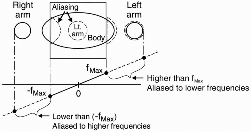 Figure 18-1. For a given FOV and gradient strength, the maximum frequency fmax corresponds to the edges of the FOV. Any part outside the FOV will experience a higher frequency. The higher frequencies outside the FOV may be aliased to a lower frequency inside the FOV. This will cause a wraparound artifact. |
For example, if the higher frequency were 2 kHz higher than (fmax), it would be recognized as 2 kHz higher than (−fmax), and therefore its information would be “aliased” to the opposite side of the image—the side of the FOV that corresponds to the lowest frequencies (Fig. 18-1).
The part of the body and arm on the left side of the patient that is outside the FOV and is exposed to a higher magnetic field will have spins oscillating at a frequency higher than (fmax). Thus, it will be identified as a structure on the right side of the patient—that side of the image associated with lower frequencies.
Likewise, the arm and body outside the FOV on the right side of the patient will experience spins oscillating at frequencies lower than (−fmax) and will also be incorrectly recognized by the computer. For example, if the lower frequency were 2 kHz lower than (−fmax), it would be recognized as 2 kHz lower than (fmax), and its information would be “aliased” to the opposite side of the image—the side of the FOV that corresponds to the higher frequencies. This process is also called wraparound—the patient’s arm gets “wrapped around” to the opposite side.
The computer can’t recognize frequencies outside the bandwidth (which determines the FOV). Any frequency outside of this frequency range is going to get “aliased” to a frequency that exists within the bandwidth. The “perceived” frequency will be the actual frequency minus twice the Nyquist frequency.
f (perceived) = f (true) −2f (Nyquist)
Why then do we usually see wraparound in the phase-encoding direction? Remember that the number of phase-encoding steps is directly related to the length of the scan time. The phase-encoding steps can be lowered by shortening the FOV in the phase-encoding direction versus the frequencyencoding direction also known as rectangular FOV (see Chapter 23). If the FOV is shortened too much in this direction versus the actual extent of the body then wraparound will occur. Figure 18-2 contains an example of wraparound.
It can be seen along the x and y directions, as with spin-echo imaging.
It can also be seen along the slice-select (phase-encoded) direction at each end of the slab (e.g., the last slice is overlapped on the first slice, as in Figs. 18-3 and 18-4).
Example
Suppose the frequency bandwidth is 32 kHz (±16 kHz). This means that if we’re centered at zero frequency, the maximum frequency fmax = +16 kHz and minimum frequency (−fmax) = −16 kHz (Fig. 18-1). If we have a frequency in the arm (outside
the FOV) of + 17 kHz, the perceived frequency will be
the FOV) of + 17 kHz, the perceived frequency will be
Now, the arm, which is perceived as having a frequency of −15 kHz (rather than +17 kHz), will be recognized as a structure with a very low frequency—only 1 kHz faster than the negative end frequency of the bandwidth—and will be identified on the opposite side of the image, the low-frequency side.
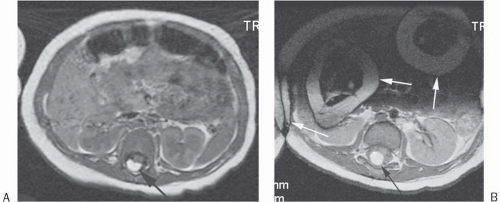 |
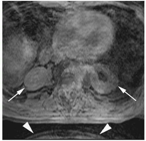 Figure 18-3. 3D gradient-echo T1 image without gadolinium of the abdomen shows slice direction aliasing with the kidneys appearing to be in the lungs (arrows). Also note that there is aliasing in the phase-encoding direction (anteroposterior) from the inferior abdominal image’s anterior subcutaneous tissue “wrapping around” posteriorly (arrowheads). |
Remedy. How do we solve this problem?
Surface coil: The simplest way is to devise a method by which we don’t get any signal from outside the FOV. With the patient in a large transmit/receive coil that covers the whole body, we will receive signal from all the body parts in that coil, and those parts outside the FOV will result in aliasing. But
if we use a coil that only covers the area within the FOV, we will only get signal from those body parts within the maximum frequency range, and no aliasing will result. This type of coil is called a surface coil. We also use a surface coil to increase the signal-to-noise ratio (SNR).
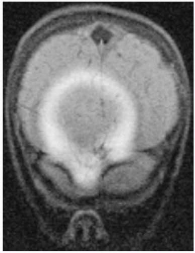
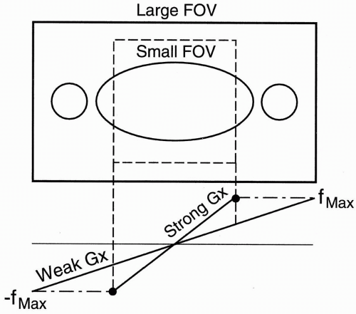
Figure 18-5. To avoid aliasing, increase the FOV.
Increase FOV: If we double the FOV to include the entire area of study, we can eliminate aliasing. To do so, we have to use a weaker gradient. The maximum and minimum frequency range will cover a larger area, and all the body parts in the FOV will be included within the frequency bandwidth; therefore, no aliasing will result (Fig. 18-5). To maintain the resolution, double the matrix with a weaker gradient (Gx). The maximum and minimum frequency range will still be the same as the stronger gradient. They will just be spread out over a wider distance. Remember, to increase the FOV, we have to use a weaker gradient.
Oversampling: Two types are discussed:
Frequency oversampling (no frequency wrap [NFW])
Phase oversampling (no phase wrap [NPW])
Frequency oversampling (NFW): Frequency oversampling eliminates aliasing caused by undersampling in the frequency-encoding direction (refer to the sampling theorem in Chapter 12). Oversampling can also be performed in the phaseencoding direction by increasing the number of phase-encoding gradients.
Phase oversampling (NPW): We can double the FOV to avoid aliasing and, at the end, discard the unwanted parts when the image is displayed (Fig. 18-6). This is called no phase wrap (NPW) by some manufacturers. It is also called phase oversampling by other manufacturers. Because Ny is doubled, NEX is halved to maintain the same scan time. Thus, the SNR is unchanged. (The scan time might be increased slightly because overscanning performs with slightly more than ½NEX.) An example of this is seen in Figure 18-7.
Saturation pulses: If we saturate the signals coming from outside the FOV, we can reduce aliasing.
Chemical Shift Artifact. The principle behind the chemical shift artifact is that the protons from different molecules precess at slightly different frequencies. For example, look at fat and H2O. A slight difference exists between the precessional frequencies of the hydrogen protons in fat and
H2O. Actually, the protons in H2O precess slightly faster than those in fat. This difference is only 3.5 ppm. Let’s see what this means by an example.
H2O. Actually, the protons in H2O precess slightly faster than those in fat. This difference is only 3.5 ppm. Let’s see what this means by an example.
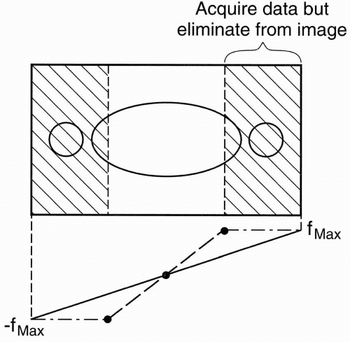 Figure 18-6. In no phase wrap, aliasing is avoided by doubling the FOV in the y direction and, at the end, discarding the unwanted part of the image. |
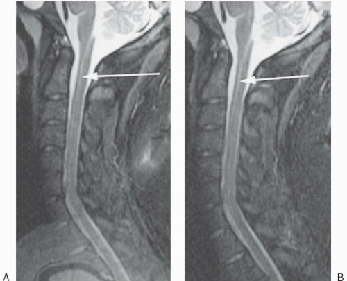 Figure 18-7. Sagittal STIR image (A) of the cervical spine with craniocaudal phase-encoding direction demonstrates aliasing of the brain onto the upper thoracic spine. (B) The same image after no phase wrap was applied. Truncation artifact is also seen (arrows). |
Example
We now have a 0.5-T magnet. The precessional frequency of protons in a 0.5-T magnet is 1/3 of a 1.5-T magnet. The frequency difference is then
Therefore, at 0.5 T, the difference in precessional frequency of the hydrogen protons in fat and in H2O is only 73 Hz. In other words, if we use a weaker magnet, we will get less chemical shift.
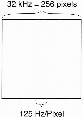
How does this affect the image? Chemical shift artifacts are seen in the orbits, along vertebral endplates, in the abdomen (at organ/fat interfaces), and anywhere else fatty structures abut watery structures. In a 1.5-T magnet, the sampling time (Ts) is usually about 8 msec. Let’s take 256 frequency points in the frequencyencoding direction.
These formulas show that the entire frequency range (i.e., bandwidth) of 32 kHz covers the whole length of the image in the x direction. Because we have the FOV of the image in the x direction divided into 256 pixels, each pixel is going to have a frequency range of its own, that is, each pixel has its own BW:

(This representation of BW on a “per pixel” basis is used by Siemens and Philips. It has the advantage of less ambiguity than the ±16 kHz designation, should the “±” be deleted.) Thus, each pixel contains 125 Hz of information (Fig. 18-8). Stated differently, the pixel bin contains 125 Hz of frequencies. Now, because fat and H2O differ in the precessional frequency of hydrogen by 220 Hz at 1.5 T, how many pixels does this difference correspond to?
 |
This means that fat and H2O protons are going to be misregistered from one another by about 2 pixels (in a 1.5-T magnet using a standard ±16 kHz bandwidth). (Actually, it is fat that is misregistered because position is determined by assuming the resonance property of water.) If pixel size δx = 1 mm, this then translates into 2 mm misregistration of fat.
MATH: For the mathematically interested reader, it can be shown that
Chemical shift
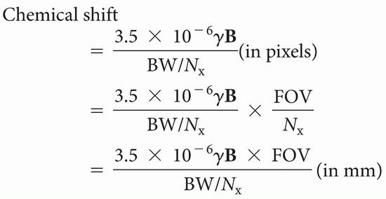
where γ = 42.6 MHz/T, B is the field strength (in T), BW is the bandwidth (in Hz), and FOV is the field of view (in cm).
Let’s now consider chemical shift artifact visually (Fig. 18-9). Remember that H2O protons resonate at a higher frequency compared with the hydrogen protons in fat. With the polarity of the frequency-encoding gradient in the x direction set such that higher frequencies are toward the right, H2O protons are relatively shifted to the right (toward the higher frequencies), and fat protons are relatively shifted to the left (toward the lower frequencies). This shifting will result in overlap at lower frequency and signal void at higher frequency. This in turn leads to a bright band toward the lower frequencies and a dark band toward the higher frequencies on a T1-weighted (T1W) or proton density (PD)-weighted conventional spin-echo (CSE) image. (On a T2W CSE, fat is dark, so the chemical shift artifact is reduced. Unfortunately, on a T2W FSE [fast spin echo—see Chapter 19], fat is bright, and the chemical shift artifact is seen.) We will see this misregistration artifact anywhere that we have a fat/H2O interface. Also remember that this fat/H2O chemical shift artifact only occurs in the frequency-encoding direction (in a conventional spin-echo image or in gradient-echo [GRE] imaging).
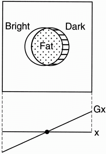 Figure 18-9. Chemical shift effect between fat and water causes a bright band toward the lower frequencies (due to overlap of fat and water at lower frequencies) and a dark band toward the higher frequencies (due to lack of fat and water signals). |
Example—Vertebral Bodies
With frequency-encoding direction—in this case, going up and down (and “up” having higher frequency) —the fat in the vertebral body would be misregistered down, making the lower endplate
bright due to overlap of water and fat and the top endplate dark due to water alone (Fig. 18-10). If we increase the pixel size, the misregistration artifact will increase.
bright due to overlap of water and fat and the top endplate dark due to water alone (Fig. 18-10). If we increase the pixel size, the misregistration artifact will increase.
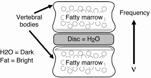 Figure 18-10. Chemical shift artifact in the vertebral endplates produces a dark band in the inferior endplates and a bright band in the superior endplates (assuming the frequencyencoding direction to be upward). |
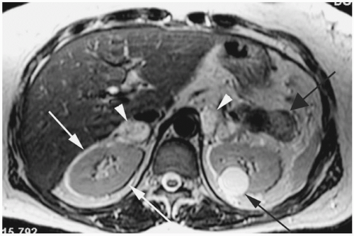 Figure 18-11. Axial T2 FSE image shows alternating bright and dark signal around the kidneys along the frequency-encoding (transverse) direction (white arrows). Patient also has bilateral pheochromocytomas (white arrowheads), a nonfunctioning islet cell tumor in the tail of pancreas (wide black arrow) and a simple cyst in the left kidney (black arrow). Patient had von Hippel-Lindau syndrome. |
Figures 18-11 through 18-15 are examples of chemical shift artifact.
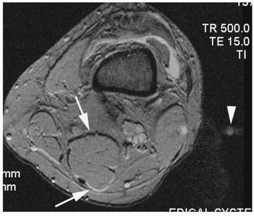 Figure 18-12. Axial T2* gradient-echo image of the knee shows first-order chemical shift (arrows) along the frequency direction (anteroposterior). Note that phase-encoding (transverse) direction “ghosting” artifact is also seen (arrowhead). A knee effusion is also demonstrated. |
Question: What factors increase chemical shift artifact?
Answer:
1. A stronger magnetic field strength
2. A lower BW:
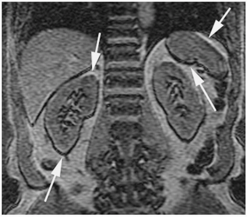 |
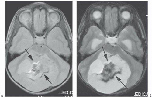 Figure 18-14. PD (A) and T2 (B) images of the posterior fossa show alternating bright and dark bands along the frequency-encoding direction (anteroposterior; arrows). Notice that the thickness of the artifact is wider in the T2 image secondary to a bandwidth (BW) of ± 4 kHz versus the PD image’s BW of ± 16 kHz. Also note that the T2 image shows only the dark band well since the fat has low signal in this CSE T2 sequence, which minimizes the amount of bright signal. Patient had mature teratoma. |
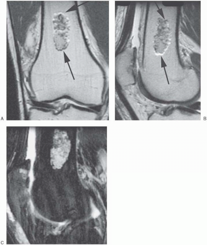 Figure 18-15.
Get Clinical Tree app for offline access
Related posts:Stay updated, free articles. Join our Telegram channel
Full access? Get Clinical Tree


|