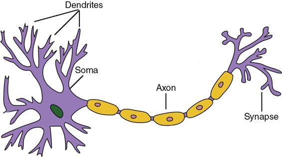
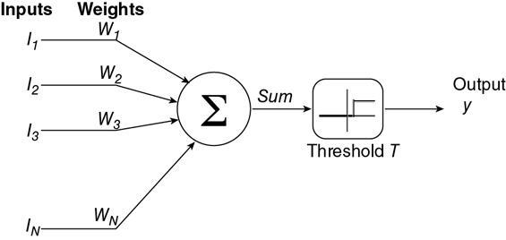
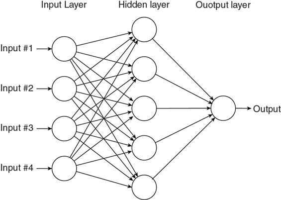
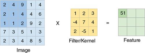
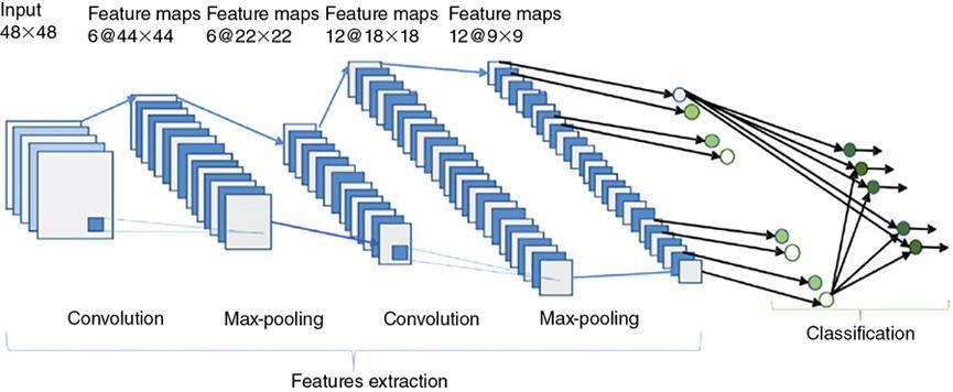
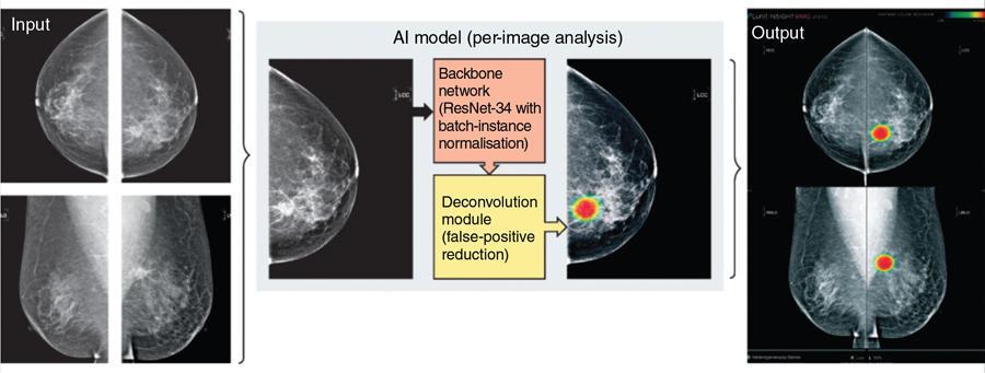
Artificial narrow intelligence

The most widely available form of AI today is artificial narrow intelligence (ANI) which refers to AI systems that are “narrow” in their capabilities. Most AI systems today are capable of performing specific tasks very well, and often more accurately or efficiently than humans, but unlike humans such AI systems are unable to perform other tasks. Take, for example, AI systems such as DeepBlue from IBM which gained a historic victory against Chess champion Gary Kasparov in the year 1997 – DeepBlue cannot perform any other task (apart from playing chess) and is hence “narrowly” intelligent. As on date, most healthcare AI systems fall into this category.

Artificial general intelligence

Humans, unlike most AI systems today, are “generally” intelligent, implying that humans can do multiple tasks reasonably well, and some tasks very well. When AI systems start exhibiting such “human-like” behaviour, they are called AGI or artificial general intelligence systems. There are several groups across the world that are currently working on such projects, and the most well known are DeepMind, which is a part of Google, and Open AI, which is an independent company working on AGI. DeepMind has already created an AI system called AlphaGo, which can learn complex strategy games by simply “observing” videos of any game and can beat the best human player in the world by learning in a matter of hours. Applications of AGI in healthcare are hypothesized but currently not available, but in the authors opinion, some of the most relevant AGI work would be useful in automating certain aspects of general practice and documentation.

Artificial super intelligence

The intersection of ANI and AGI, wherein there is an AI system that is narrowly intelligent in almost all domains and has the ability to develop narrow expertise in any domain, is referred to as an artificial super intelligence (ASI) system. While there is a great degree of debate about the very possibility of ASI, there is an ever greater degree of debate and thought that AI leaders are putting into the controlling of such a system – such a system would be infinitely more capable than human beings, and hence, it would be paramount to keep it in check to ensure that the power/tasks allocated to it do not lead to self-destruction. This is, however, conjecture as yet and seems to be several decades, if not hundreds of years away.

Biological neuron

The brain is composed of billions of interconnected neurons. Each of the purple blobs in Fig. 1.26.1 are neuronal cell bodies, and the lines are the input and output channels (dendrites and axons) which connect them. Each neuron receives electrochemical inputs from other neurons at the dendrites. If the sum of these electrical inputs is sufficiently powerful to activate the neuron, it transmits an electrochemical signal along the axon and passes this signal to the other neurons whose dendrites are attached at any of the axon terminals. It is important to note that a neuron fires only if the total signal received at the cell body exceeds a certain level. The neuron either fires or it does not; there are not different grades of firing – the so-called “all or none” phenomenon.

The human brain is composed of these interconnected electrochemical transmitting neurons. From a large number of extremely simple processing units (each performing a weighted sum of its inputs, and then firing a binary signal if the total input exceeds a certain level), the brain performs extremely complex tasks.

History of neural networks and the perceptron

The basis of neural networks or deep learning (DL) stems from the inner working of brain neurons. The studies date back to 1943 when two scientists Warren McCulloch, a neurophysiologist, and Dr Walter Pitts, a mathematician first portrayed to mimic the neuron interaction with a simple electrical circuit. Donald Hebb in 1949 then took the idea forward in his book “The organization of Behavior” proposing that neural pathways strengthen over each successive use, especially between neurons that tend to fire at the same time. This began the journey of quantifying the brain processes. Donald Hebb also proposed a method called Hebbian Learning that essentially says that “Cells that fire together, wire together”. Based on Hebbian Learning, the first Hebbian network was first built successfully at the Massachusetts Institute of Technology in 1954. Around this time, Frank Rosenblatt in 1958 first coined the term Perceptron while he was trying to simplify the neuron interaction in brain using a mathematical model based on McCulloch–Pitts neuron, calling it Mark I Perceptron (Fig. 1.26.2). The M-P neuron takes in inputs, takes a weighted sum and returns 0 if the resultant is below the threshold and 1 otherwise.

The advantage of Mark I Perceptron was that the weights could be “learned” through successive passed inputs, reducing the difference between the output and the desired output. But the disadvantage was that it could only learn linear relationships. With many ups and downs in this research direction with intermediate introduction of Hopfield network in 1982, it was only after the rediscovery of backpropagation learning algorithm by Rumelhart, Hinton and Williams that took the community with storm. Backpropagation along with gradient descent forms the building block of today’s artificial neural networks (ANNs).

The perceptron is a mathematical model to imitate the working of brain neurons. It takes inputs, applies a weighted summation and passes through an activation function, which can be a nonlinear function (tan h, sigmoid) as well and gives the final output. The error in the desired output and the model’s output is termed as error. This error is then propagated back to the input, and the weights of the perceptron are updated.

Multilayered perceptron (or neural network)

Using multiple perceptrons and stacking multiple layers of perceptron besides each other forms the multilayered perceptrons. The inputs enter the multilayered perceptron through the input layer, which is passed through the hidden layer made of multiple perceptrons. Each perceptron in the input layer sends multiple signals. One signal goes to each perceptron in the next layer. The output of the hidden layer is then passed through the output layer to get the final output. Each perceptron may or may not contain a nonlinear activation function and uses different weights for each signal. The weights of each perceptron are updated using errors computed between the output of the model and the desired output by using backpropagation algorithm. Multilayered perceptron is also called as a neural network. This is illustrated in Fig. 1.26.3.

Convolutional neural networks

To understand a convolutional neural network, we first need to understand what an image is. To humans, an image is simply an image of an object or person, with multiple colours, emotions and thoughts. To computers, it is simply a table (or matrix) with numbers (pixel values). This comparison is visible in Fig. 1.26.4.

A classic use of a CNN is for an image classification task, where an input image is classified into predefined categories, for example, looking at a human image and classifying it into male or female. ANNs (described earlier) can certainly be used to perform this task, but there are a lot of reasons we do not use them:

Note that CNNs are nothing but neural networks (or multilayer perceptrons) made up of convolutional layers (or Conv layers) which are based on the mathematical function of convolution. A Conv layer consists of some filters which are nothing but 2D matrices. The process of convolution is as follows (Fig. 1.26.5):

A Conv layer performs the aforementioned process iteratively on all locations of the image and outputs another matrix which is called a feature. These features are then passed through other Conv layers till the output layer classifies the image into one of the classes/categories defined. This iterative process of “learning” features is at the heart of all AI today (Fig. 1.26.6).

Classification

The most common type of AI available today for radiology is a classification algorithm. Classification algorithms, or simply classifiers, take an image or a group of images as input and then output whether a particular finding, disease or pathology is present in the input images or not. Classifiers can be single-label or multilabel classifiers. Examples of classification algorithms are those which diagnose the presence of tuberculosis in chest X-rays (2), critical findings on head CT scans (3) or even whether a particular chest X-ray is normal or abnormal (4). Essentially, any AI algorithm that claims to give a “diagnosis” falls into this category. As you may notice, these examples refer to those which give binary output (TB vs no TB, normal vs abnormal), there may also be algorithms which give output as a continuous variable, for example, algorithms that take a hand X-ray as input and output the patient’s bone age by either Tanner–Whitehouse (TW3) method or Greulich and Pyle (GP) method.

Localization

Localization refers to the ability of an AI algorithm to discern where a particular finding (from the classification algorithm) resides on the image. It is generally superimposed on a classification algorithm with the intent of attempting to “see” what the key driver of the AI’s output has been. For example, in algorithms that automatically detect malignant lesions on mammography images, when the algorithm also gives the location of the malignant lesion – it is referred to as a localization or detection algorithm (Fig. 1.26.7).

Related posts:

Syndromes and rare diseases in neck Image guided nerve blocks and sympathectomies Bleeding diathesis The anterior skull base and the first cranial nerve – imaging anatomy and pathology Imaging of masticator space Basic medical sciences for radiologists

Stay updated, free articles. Join our Telegram channel

Join