div class=”ChapterContextInformation”>
16. Hemodynamic Aspects of Vessel Wall Imaging: 4D Flow
Keywords
4D flowMRIBlood flowHemodynamicsWall shear stressPulse wave velocityVessel wallIntroduction
Cardiovascular MRI has undergone substantial developments over the last decades and offers capabilities for evaluating cardiac anatomy and function including the assessment of vascular anatomy and blood flow dynamic. Phase contrast (PC) MRI can be used to measure and quantify pulsatile blood flow in the human vascular system.
The basic principle has already been introduced by Carr and Purcell in 1954 who reported the observation of coherent motion on the MR signal [1] and by Hahn in 1960 who proposed to use nuclear precession to measure the velocity of sea water by means of phase shifts produced by magnetic field gradients [2]. Two decades later, Grant and Back were among the first to investigate the possibility of measuring flow velocity with MRI [3]. They called the technique “NMR rheotomography” and were visionary by remarking that “rheotomography may prove to be particularly useful for the noninvasive diagnosis of cardiovascular defects.” Nearly 40 years later, many groups worldwide are using MRI flow measurements for the noninvasive diagnosis of cardiovascular defects. The first in vivo velocity map images and applications were reported in the early 1980s [4–7]. The initial measurement of a through-plane velocity profile in a two-dimensional (2D) slice of water flowing through a glass U-tube has evolved, and 2D and time-resolved (ECG-gated “CINE” imaging) PC-MRI has become available on all modern MR systems and is an integral part of clinical protocols assessing blood flow in the heart and large vessels [8–10]. More recently, the combination of CINE PC-MRI with three-dimensional (3D) spatial encoding and three-directional velocity encoding (termed “4D flow MRI”) has made possible measurements of 3D blood flow dynamics in a 3D volume and over time (4D = 3D + time) [11–13].
This chapter will review the journey from simple 2D to 4D flow MRI for the advanced quantification and visualization of hemodynamic measures in vessel wall disease. We will describe the fundamental concepts of 4D flow MRI in terms of acquisition, data processing, as well as its applications to the assessment of altered blood flow dynamics in vascular diseases. A special emphasis is on the potential of 4D flow MRI to quantify important characteristics of the vessel wall such as wall shear stress (WSS) or pulse wave velocity (PWV). The chapter will conclude with a discussion of the current role of 4D flow MRI and future directions.
Background
From 2D to 4D Flow Image Acquisition
Flow imaging with MRI is based on the phase contrast (PC) technique, which enables the acquisition of spatially registered information on blood flow velocities simultaneously with morphological data within a single MRI measurement. In current clinical routine, PC-MRI is typically accomplished using methods that resolve two spatial dimensions (2D) in individual slices and encode a single time-resolved component of velocity directed perpendicularly to the 2D slice (through-plane velocity encoding). This approach allows measurements of forward, regurgitant, and shunt flows in congenital and acquired heart disease. In MRI, magnetic field gradient coils can create linearly varying magnetic fields along all three spatial dimensions on top of the main (static) magnetic field B0. These magnetic field gradients cause spatially varying phase shifts of the source of the MRI signal (1H proton spins in the human body) depending on the location of the source along the gradient. Spins that move along the direction of the gradient, e.g., flowing blood, acquire a different phase shift than the spins in adjacent static tissue [14].
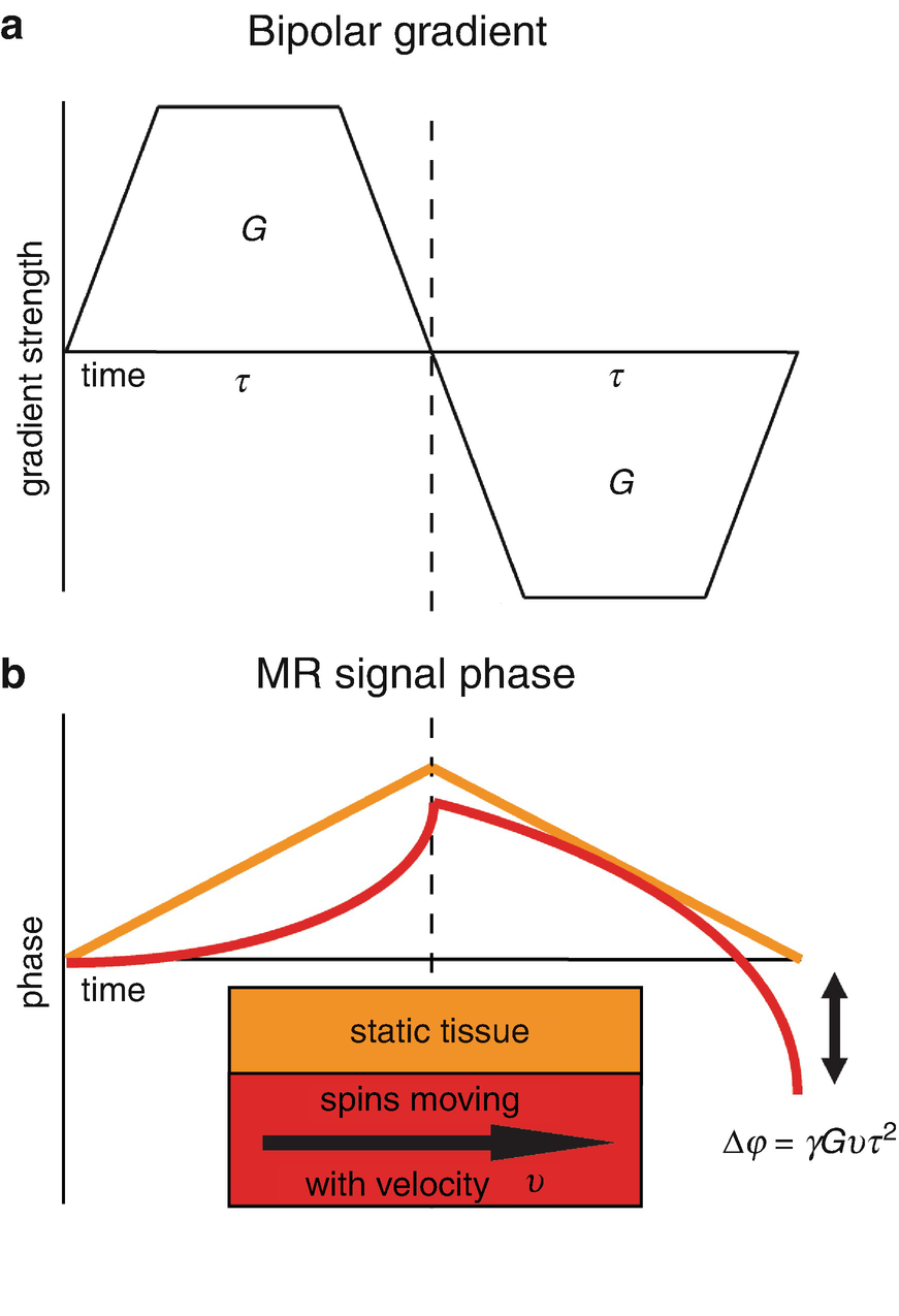
(a) A bipolar gradient that causes (b) a phase shift for moving spins compared to zero phase for static spins. The phase shift ∆φ is proportional to the gyromagnetic ratio γ, the gradient strength G, the velocity of the moving spins v, and the gradient duration τ. Note that the equation represents a simplified situation where grant ramps are ignored for then coagulation of the calculation of phase shift ∆φ
Using appropriate bipolar velocity encoding gradients, flow-dependent phase changes can be measured by playing out two acquisitions with different velocity dependent signal phase but otherwise identical sequence parameters. Subtraction of the two resulting phase images (i.e., calculation of phase difference images) allows for the removal of the unknown background phase and calculation of velocity images [9].
With a bipolar gradient applied to the main direction of the blood flow, single-direction (e.g., through-plane) blood flow velocity is measured. Bipolar gradients can also be subsequently applied to two or three orthogonal axes to resolved blood flow velocities in two or three dimensions [15, 16].

In 2D CINE PC-MRI, ECG triggering over multiple R-R intervals is used to acquire a series of time frames over the cardiac cycle. For each time frame, reference MRI raw data (k-space) lines (without bipolar gradient) and velocity encoded k-space lines (with bipolar gradient) are acquired. The number of k-space lines acquired for each time frame is determined by the segmented k-space or turbo field echo factor. After completion, phase contrast magnitude anatomical images and phase difference containing the velocity information are reconstructed. The figure illustrates 2D PC-MRI acquisition at the site of the aortic valve peak systole (top) and diastole (bottom)
For over three decades, 2D CINE PC-MRI has been widely used for flow quantification in the aorta [19], the carotid arteries [20] and the intracranial vessels [21]. For routinely used 2D CINE PC-MRI, a slice for a 2D measurement is manually positioned perpendicular to a vessel, and blood flow velocity is encoded in one direction through the 2D slice. However, placement of the acquisition plane remains challenging and can lead to the underestimation of peak velocities if misplaced or not orthogonal to the flow of interest. This is a common occurrence in cases involving complex flow and where changes in flow direction occur throughout the cardiac cycle, such as with valvular stenosis, valvular regurgitation, complex congenital heart disease, or aneurysms. These challenges can be addressed by three-dimensional (3D) PC-MRI with three-directional velocity encoding which can provide comprehensive information on the in vivo 3D blood flow dynamics with full volumetric coverage of the vascular region of interest. Wigström et al. were the first to implement a high spatial resolution and electrocardiogram (ECG)-gated 3D cine phase contrast pulse sequence, currently known as 4D flow MRI (4D = 3D+ time over the cardiac cycle, flow = three-directional velocity encoding) [22].
4D Flow Acquisition Methods and Techniques
Data Acquisition

Acquisition of 4D flow MRI data and analysis of hemodynamic metrics in the thoracic aorta of a healthy subject. (a) ECG synchronized 4D Flow MRI data acquisition. For each time frame, four 3D raw data sets are collected to measure three-directional blood flow velocities (vx, vy, vz) with a reference scan and three velocity encoded acquisitions. k-space segmentation is used to collect a subset (NSeg) of all required raw data (k-space) lines for each time frame. The selection of NSeg determines the temporal resolution and total scan time. (b) 4D flow data comprises information along all three spatial dimensions, three velocity directions, and time in the cardiac cycle. (c) A 3D phase contrast angiogram (3D PC-MRA) can be calculated from 4D flow MRI data to aid visualization and provide a basis for the 3D segmentation of the aorta (orange rendering of aorta). Systolic streamlines allow for visual assessment of flow patterns and placement of analysis planes for retrospective flow quantification. Calculation of a systolic velocity maximum intensity projections (MIP) provides an overview over systolic velocity distribution and allows for volumetric quantification of peak systolic velocity (location of peak velocity is indicated by black circle in the ascending aorta). Advanced vessel wall characteristics can be derived such as systolic 3D wall shear stress (WSS) vectors along the aorta. AAo ascending aorta, DAo descending aorta
It should be noted that increasing 4D flow spatial resolution by reducing voxel size is possible but is accompanied by a decrease in signal-to-noise ratio (SNR) and thus image quality. Moreover, for volumetric acquisitions such as 4D flow MRI, scan times increase cubically with isotropic voxel size reduction.

(a) Bipolar gradients of higher strength and thus a low-VENC cause (b) aliasing (black arrow) in the phase difference images of the aorta, whereas aliasing is avoided when VENC is tailored to the expected maximum velocity in (c). (d) At a high VENC, the sensitivity to changes in aortic velocities is decreased. AAo ascending aorta, DAo descending aorta
In Fig. 16.4, the principle of VENC is shown for through-plane 2D phase difference images of the aorta with severe velocity aliasing when the VENC is selected too low (high bipolar gradient). Unaliased flow velocities are achieved when the VENC is tailored to the expected maximum velocity (lower bipolar gradient).
Typical (ranges of) scan parameters for three different anatomical regions
k-space segmentation (turbo field echo factor) | (Isotropic) spatial resolution (mm3) | Temporal resolution (ms) | VENC (cm/s) | |
|---|---|---|---|---|
Heart/aorta | 1–3 | 2.0–3.0 | 20–60 | 150–400 |
Carotid | 2–3 | 0.8–1.4 | 40–60 | 100–150 |
Intracranial | 2–4 | 0.5–1.2 | 40–80 | 70–150 |
Data Acquisitions: Imaging Acceleration Techniques
Long scan times on the order of 10–20 minutes have previously relegated 4D flower MRI to the realm of research. However, current implementations are quickly approaching clinically feasible scan times, on the order of 2–8 minutes. Methodological improvements include echo planar imaging (EPI), where multiple Cartesian readouts are acquired after one excitation to obtain high spatial resolution [29]. Additional imaging acceptation is based on parole imaging such as sensitivity encoding (SENSE) [30, 31], generalized autocalibrating partially parallel acquisitions (GRAPPA) [32], k-t acquisition speed-up techniques (k-t BLAST) [33, 34], k-t GRAPPA [35], k-t principal component analysis (k-t PCA) [36, 37], and CIRCUS [38]. Another promising technique to accelerate 4D flow MRI is compressed sensing where data is acquired in a sparse and random manner followed by nonlinear recovery of data [39, 40]. For example, aortic 4D flow MRI is now possible with a scan time of less than 2 minutes without substantial degradation of image quality [41].
Data Acquisitions: Non-Cartesian Sampling
An alternative technique that is increasingly used to accelerate 4D flow MRI is radial data sampling combined with undersampling (e.g., PC-VIPR – vastly undersampled isotropic projection reconstruction [42]). Radial sampling has two important advantages over Cartesian readouts: (1) sparse sampling results in streak image instead of fold-over artifacts which allows for higher undersampling factors [42] and (2) the center of k-space is continuously sampled and results in insensitivity to subject motion [43]. As an alternative, spiral k-space sampling can cover the entire k-space uniformly and rapidly [44], allowing for rapid 4D flow MRI velocity measurements [45–47]. However, both radial and spiral sampling are sensitive to eddy current effects which require efficient correction strategies, and image reconstruction is more computationally demanding. Alternatively, radial- and spiral -like trajectories can be implemented on a Cartesian grid, called pseudo-radial and pseudo-spiral trajectories [48, 49]. For example, a recently reported combination of pseudo-Cartesian acquisition schemes coupled with compressed sensing for imaging acceleration has shown great potential for fast and robust pediatric 4D flow MRI [50].
Data Acquisitions: Respiratory Control (Gating, Self-Gating)
For cardiothoracic and abdominal applications, methods for respiration control are needed to prevent image deterioration due to respiratory motion. Early efforts in MRI have focused on gating of the respiratory signal using bellows [51] or navigator echoes in a longitudinal beam placed on the diaphragm [52]. Most methods are based on accepting data in the expiration phase when chest motion is minimal and rejecting data acquired in the inspiration phase when the chest is moving. Other strategies minimize respiration-related image degradation by respiratory ordered phase encoding (ROPE): measurements at inspiration are attributed to the center of k-space, whereas the measurements at expiration are attributed to the edges of k-space [53]. Such strategies have been successfully implemented for 4D flow MRI [54] in combination with navigator gating [55]. Other promising approaches employ self-gating techniques, e.g., cross-correlation with reference breathing motion to identify different respiratory phases [56] or extracting respiratory and cardiac motion signals from additional and repeatedly sampled central k-space data [57].
4D Flow Analysis Methods and Techniques
Preprocessing and Phase Offset Error Corrections
4D flow MRI data are affected by systematic velocity encoding errors caused by magnetic field inhomogeneity, concomitant magnetic fields (Maxwell terms) [58], and eddy currents [59, 60]. Correction of these errors typically includes the identification of image regions that contain static tissue in order to estimate the spatial distribution of background phase offsets (using a first- or second-order fit to the static tissue phase difference data) [61]. Background phase errors can subsequently be removed by subtraction of the estimated offset from the entire velocity data [62].
It is common in 4D flow MRI that the VENC setting is lower than the maximum velocity in the measurement and that velocity aliasing occurs. With the assumption that adjacent pixel velocities in the temporal or slice direction should not differ more than VENC [28], aliased velocities can be automatically detected and corrected [63].
Visualization and Quantification of 4D Flow MRI Hemodynamics
For effective visualization of the information encoded in the large 4D flow MRI data sets (see Fig. 16.3b), many methods have been developed and include velocity vector display in three-dimensional space [64, 65] streamlines [66, 67], and path lines/particle traces [67].
Figure 16.3c illustrates 4D flow MRI-based evaluation of fundamental (flow, peak velocity) and advanced hemodynamic metrics (wall shear stress, WSS) based on a single acquisition. Visualization of the vascular geometry can be achieved from a 4D flow acquisition by generating a non-contrast 3D PC-MR angiogram (MRA). A surface rendering of the vascular structure of interest (see Fig. 16.3c, left) allows for regional orientation, analysis, and flow visualization. For qualitative visualization of 4D flow MRI data, 3D streamlines or time-resolved 3D path lines can be used for flow pattern visualization. Streamlines represent the instantaneous blood flow vector field for a single cardiac time-frame. For example, Fig. 16.3c illustrates the use of systolic 3D streamlines to visualize the spatial distribution and orientation of blood flow velocities. Color-coding by velocity magnitude facilitates the visual identification of regions with high systolic flow velocities. For visualization of the temporal evolution of 3D blood flow, time-resolved path lines are the method of choice. Time-resolved path lines are best viewed and displayed dynamically (movie mode) to fully appreciate the dynamic information and changes in blood flow over the cardiac cycle. It is important to differentiate between streamlines and path lines since the former represents the instantaneous tangent to the velocity vector at a given time in the cardiac cycle (e.g., peak systole), while the latter resemble traces of the dynamically time-varying blood flow over the cardiac cycle. 4D flow MRI can also be used to derive volumetric and maximum intensity projections (MIPs) of peak velocity for easy volumetric identification of peak flow velocities (see Fig. 16.3c).
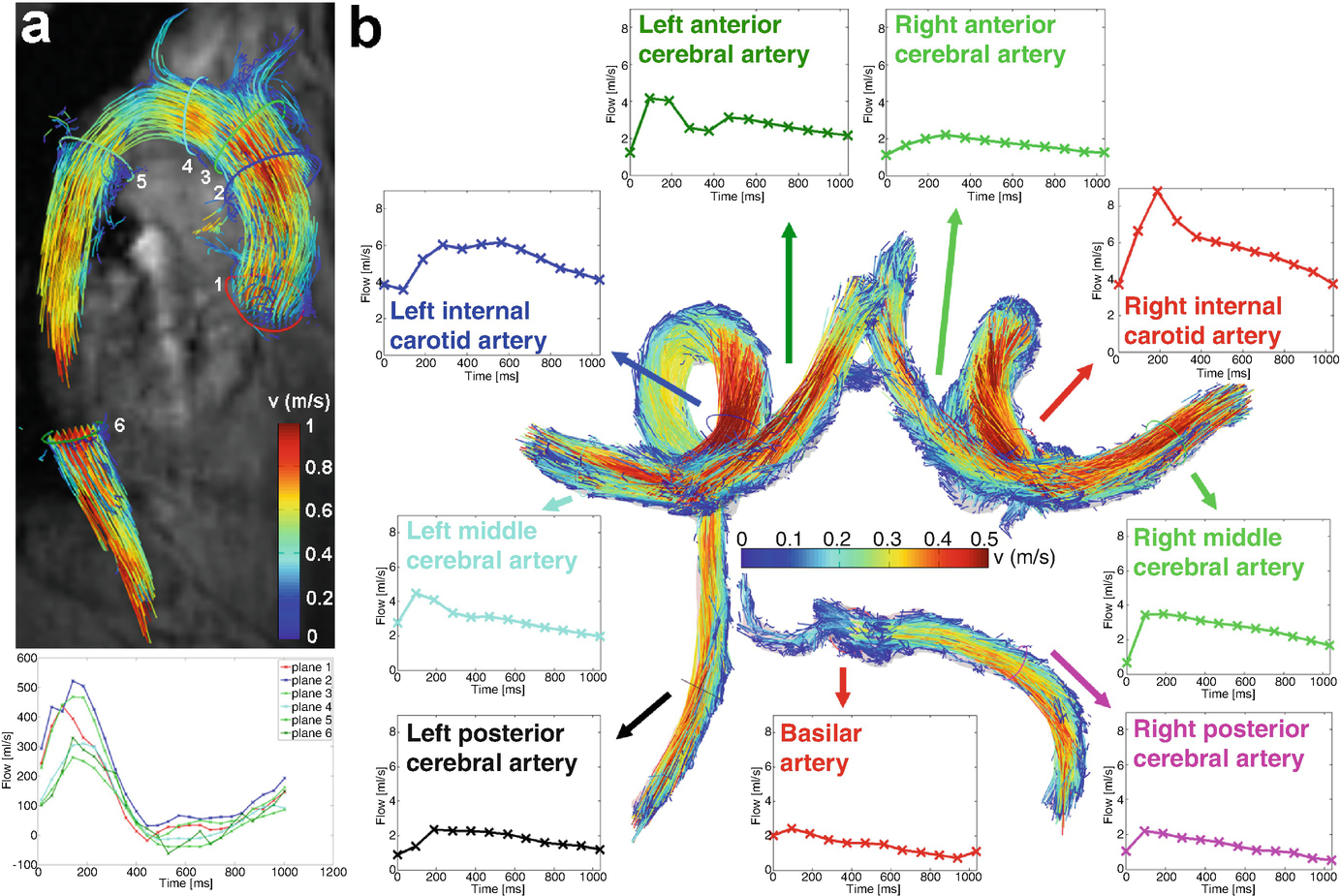
(a) 3D flow visualization (path lines and with flow quantification in perpendicular 2D analysis planes at standardized locations in the healthy aorta) [68]. (b) 3D segmentation and flow visualization in the circle of Willis of a healthy volunteer. Flow quantification based on perpendicular 2D analysis planes allows for the systematic assessment of blood flow over the cardiac cycle in the entire circle of Willis
Advanced Hemodynamic Vessel Wall Metrics
In addition to 3D blood flow visualization and planar flow quantification, 4D flow MRI offers the opportunity to derive advanced hemodynamic measures such as vorticity [69, 70] and helicity [71, 72], wall shear stress (WSS) [73, 74], pressure gradients [75, 76], viscous energy loss [77, 78], turbulent kinetic energy [79, 80], or pulse wave velocity (PWV) [81, 82]. This article will focus on the two parameters most relevant for vascular wall characterization: PWV and WSS.
Pulse Wave Velocity
It is well understood that arterial vascular stiffening (i.e., reduction of vessel wall elasticity) can lead to atherosclerosis and the development of vessel wall abnormalities and atherosclerotic plaques. Pulse wave velocity (PWV), the best known surrogate measure for arterial stiffness, is the speed of the pulsatile pressure wave that propagates along arteries in a heartbeat [83–85]. PWV is determined by the elastic modulus of the vessel, the vessel wall thickness, the vessel radius, and the density of blood (Moens-Korteweg equation) [85]. Thus, increased PWV is directly associated increased elastic modulus (i.e., stiffening) and vessel wall thickness. Both processes occur in early atherosclerosis, and PWV is thus considered an important indicator for the onset of this disease. A meta-analysis revealed that increased PWV and thus reduced aortic compliance is a strong predictor of future cardiovascular events and all-cause mortality. Moreover, an increase in aortic PWV by 1 m/s corresponded to an age-, sex-, and risk factor-adjusted risk increase of ca. 15% in total cardiovascular events [86]. Reliable measurement of PWV is thus of high interest, e.g., for monitoring vessel compliance during therapy [87, 88].
Carotid-femoral PWV using tonometry is the current reference standard to measure aortic compliance [89]. This method, however, is prone to errors and does not focus on regional compliance. Time-resolved 2D CINE PC -MRI provides a noninvasive estimate of PWV based on flow waveform measurements in analysis planes and allows focusing on the region of interest in patients, e.g., the thoracic aorta or carotid arteries [90–92]. Transit-time (TT) methods are typically employed to calculate temporal differences of specific flow waveforms features, e.g., timing differences of the foot of the waveform between two locations with known distance, as first described in 1989 for the aortic arch [93]. The accuracy of PWV quantification can be improved by adding velocity encoding directions [81] or using multiple measurement locations [94, 95].
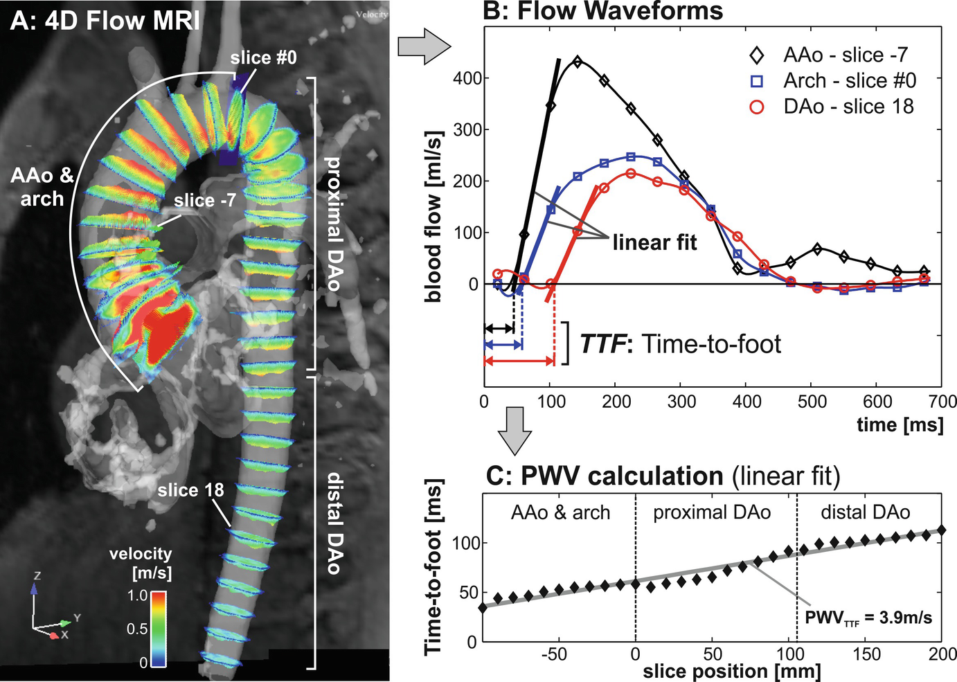
Derivation of aortic pulse wave velocity from 4D flow MRI: (a) flow curves are automatically extracted in multiple planes along the aortic centerline. An initial plane #0 is positioned at the proximal asking aorta. Subsequently, all other 2D analysis planes will be positioned downstream in fixed intervals. (b) For each analysis plane, flow-time curves are calculated and the time-delay between adjacent planes is derived. (c) Aortic PWV (in m/s) is determined by a linear fit from data of the entire aorta. AAo: ascending aorta, DAo: descending aorta
Wall Shear Stress
 that contains the velocity gradients in all directions at the wall, with the viscosity of blood. As schematically illustrated in Fig. 16.7 (top), initial studies have employed 4D flow MRI to quantify regional time-resolved WSS based on 2D analysis planes [105]. The variation of WSS direction over the cardiac cycle can be used to calculate the oscillatory shear index (OSI) [106]. More recently, methods have been developed to compute volumetric 3D WSS along the 3D surface of the entire aorta, carotid or intracranial vasculature, or aneurysms (Fig. 16.7, bottom) [74, 107–109]. For the aorta, a method for the quantification of turbulent WSS variation was recently developed [110].
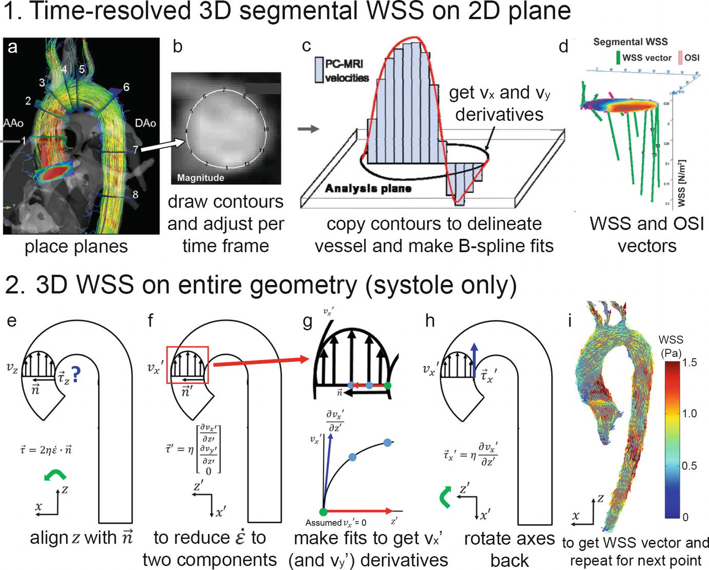
(1) 3D segmental WSS in 2D planes. (a) Planes are placed perpendicularly to the aorta measured with 4D flow MRI, (b) contours are manually drawn to delineate the vessel wall and to define the segments for WSS calculation, (c) B-spline fits through the vx and vy velocities are created to derive the gradients at the wall that after multiplication with blood viscosity, (d) yield the WSS vectors in the plane. When repeated for all time frames, OSI can be calculated. (2) 3D WSS on the entire aorta surface. (e) At each point along the vessel wall, the z-axis is aligned with the inward normal vector, and with the assumption that there is no velocity through the wall, the deformation tensor is reduced from nine components to two (f). Spline fits along the x and y velocities along the normal vector yield the vx and vy derivatives. After multiplication with viscosity and rotation back to the original axes system, the local WSS vector is obtained
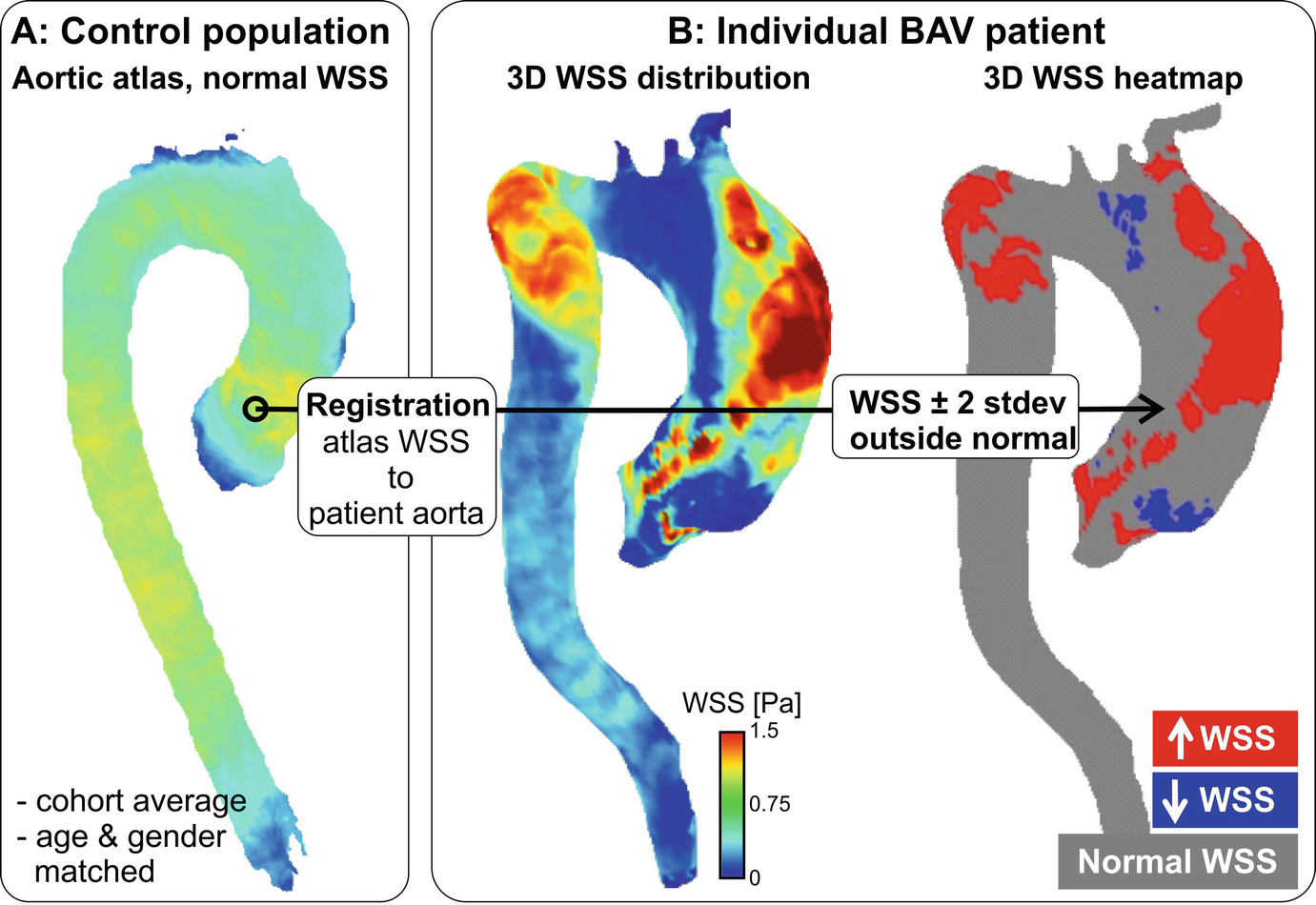
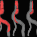
Patient-specific WSS heatmaps. (a) A 3D cohort-averaged WSS map of a control cohort (“WSS atlas”) is used as reference to provide mean, median, and normal confidence intervals (CI = ± 2 standard deviations, SD) of the normal physiologic aortic WSS distribution. (b) After delineating the regions of abnormal WSS for an individual patient, defined as values outside the CI, heatmaps of abnormally elevated or decreased WSS are created
It should be noted that the discrete nature of the 4D flow MRI measured velocity field will result in a systematic underestimation of WSS. This is a common limitation of the technique. While absolute accuracy when assessing WSS in vivo is challenging, the relative pattern of expression (and magnitude) can reliably be inferred, especially if scan parameters and the procedure for WSS estimation are consistent between study populations [113, 114].
4D Flow MRI in Vessel Wall Disease: From Head to Toe
Head
In clinical practice, transcranial Doppler ultrasound is routinely used for cerebrovascular flow measurements. However, the technique is operator-dependent and limited by the acoustic windows of the head. 2D PC-MRI can provide reliable flow measurements in large intracranial arteries and veins, not limited by location. However, challenges for using 2D PC-MRI for flow measurement include small and tortuous vessels [115], complex vascular anatomy, and need for the manual placement of 2D imaging planes in multiple vessel segments. As an alternative, 4D flow MRI is increasingly used to assess cerebrovascular 3D blood flow [116, 117]. Emerging applications include the hemodynamic evaluation of intracranial aneurysms, arteriovenous malformations (AVM), and intracranial atherosclerotic disease (ICAD). Several groups have reported the successful measurement and evaluation of flow and WSS in intracranial aneurysms in patient feasibility studies [107, 118–121], indicating the potential of flow MRI to assist in the classification of individual aneurysms pre-intervention.
Arteriovenous Malformations (AVMs)
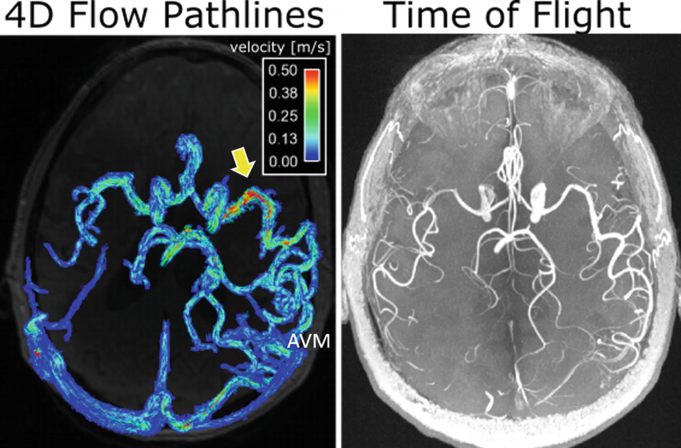
Intracranial 4D flow MRI (left) and time-of-flight (TOF) 3D angiogram (right) in a 62-year-old male patient with a large cerebral AVM (Spetzler-Martin grade = 3). The dense AVM vascular network and high flow velocity in a main AVM feeding artery (arrow) can clearly be appreciated
Intracranial Atherosclerotic Disease (ICAD)
Intracranial atherosclerotic plaques can alter local and global hemodynamics (particularly proximal or distal to stenosed vessels). Currently, intracranial hemodynamic disturbance in patients with ICAD is primarily assessed using transcranial Doppler ultrasound. Few studies have been performed to characterize the 3D blood flow disturbance and flow redistribution across the major cerebral arteries in patients with ICAD. An early study by Hope et al. reported that TOF MRA overestimated the degree of stenosis and that 4D flow MRI velocity measurements could improve accuracy of diagnosis, when compared to catheter angiography [119]. It should be noted that current flow imaging techniques (2D and 4D) are limited by insufficient spatial resolution for the characterization of blood flow at sites of critical or severe stenosis. Instead, post-stenotic flow is typically used to represent the regional flow in the stenotic artery. Higher magnetic field (7 Tesla) with increased spatial resolution may be required for improved flow assessment in the smaller vessels [125].
Intracranial Aneurysm
A large number of studies investigating flow patterns in intracranial aneurysms were based on computational fluid dynamics (CFD) techniques in conjunction with subject-specific geometries extracted from medical images [126–129]. Findings from these studies revealed a wide variety of complex intra-aneurysmal flow patterns that were strongly dependent on patient-specific vascular geometry. In addition, a number of studies showed that changes in WSS along the wall of intracranial aneurysms may be associated with risk of aneurysm growths or rupture [73, 107, 121]. However, CFD has limitations such as assumptions concerning blood properties, boundary conditions, and vessel properties [129–131]. As an alternative, 4D flow MRI is increasingly used to assess intra-aneurysmal 3D hemodynamics in vivo. Several groups have reported the successful measurement and evaluation of intra-aneurysmal flow and WSS in patient feasibility studies [73, 116, 119, 132–137], indicating the potential of flow MRI to assist in the classification of individual aneurysms pre-intervention.
Neck
Carotid artery stenosis is a leading cause of ischemic stroke, and detailed insights into the causes for the development of atherosclerosis at this site are of interest. Among other risk factors, it is assumed that the development of atherosclerosis in the naturally bulbic ICA is related to local hemodynamic conditions such as flow deceleration or recirculation associated with reduced and oscillating WSS [138]. Particularly, low absolute WSS and high OSI are hypothesized to determine the composition of atherosclerotic lesions and the development of high-risk plaques [99, 102]. Since blood flow through the carotid bifurcation is complex with nonsymmetric flow profiles, the full three-directional velocity information by 4D flow MRI can be useful for a complete in vivo assessment of the segmental distribution of WSS.

Three-dimensional (a) wall shear stress and (b) wall thickness carotid bifurcation maps averaged over 20 subjects with plaques. In (c) the correlation between WSS and WT is shown with color-coding for the density of the points
4D flow MRI-derived WSS quantification could thus be a valuable technique to assess the individual risk of flow-mediated atherosclerosis and carotid plaque progression.
The assessment of PWV in the carotid arteries as a measure of vessel stiffness (and thus atherosclerotic burden) is challenging due its small size that necessitates high spatial and temporal resolution [147]. It is thus challenging to derive PWV using 4D flow MRI in the carotid arteries. For the determination of local PWV in the carotid arteries, the temporal resolution of through-plane 2D CINE PC-MRI was recently drastically improved by compressed sensing acceleration [148]. These novel acquisition strategies hold promise for future applications of either 2D or 4D flow MRI-derived PWV.
Thorax
Cardiothoracic 4D flow imaging is typically performed as part of a standard-of-care aortic/pulmonary imaging protocol, which includes additional MRI techniques for the assessment of cardiac function and wall motion (CINE imaging), aortic and pulmonary dimensions and geometry (MR angiography), as well as aortic and pulmonary valve morphology and dynamics (CINE imaging). The combination with 4D flow MRI provides a comprehensive assessment of aortic/pulmonary structure and function. These data have contributed to the understanding of the development of vessel wall abnormalities (atherosclerosis, aortic dilation, aneurysm) as a consequence of thoracic vascular diseases such as aortic valve diseases (stenosis, insufficiency, congenital bicuspid aortic valve (BAV)), aortic coarctation, or Marfan syndrome.
Aortic Valve Disease and Aortopathy
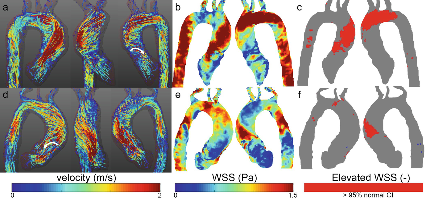
Velocity and WSS in two patients with a stenosed bicuspid aortic valve. (a, d) Peak systolic velocity path lines showing right-handed helical flow (top) and left-handed helical flow (bottom). Vortex flow can be seen as well (white arrows). (b, e) Stenotic flow leads to high wall shear stress on the right-anterior aortic wall (top) and left-posterior wall (bottom) which can be concisely visualized by elevated WSS heatmaps (c, f)
Related posts:

Stay updated, free articles. Join our Telegram channel

Full access? Get Clinical Tree


