Fig. 26.1
Rationale for measuring bone in children. Bone properties in children may predict childhood fractures as well as osteoporosis and fractures during adulthood
Assessing bone deficiency in children is fundamentally different from assessing osteoporosis in elderly adults. Since children are growing, low bone mass reflects deficient bone accrual, rather than excessive bone loss. The bone accumulated during childhood determines the peak bone mass reached in early adulthood. Peak bone mass is one of the most important determinants of the risk of osteoporosis.
Genetic susceptibility to osteoporosis and fractures manifests in early childhood. Even before puberty, girls and their mothers share similar bone traits [6]. In addition, genes associated with normal variations in bone mass in the elderly may be related to variations in bone density in children [7]. Finally, measures of bone appear to “track” during growth, with bone mass at a younger age predicting bone mass at older ages. Dual-energy x-ray absorptiometry (DXA) measures of bone mineral content and bone mineral density track over at least a 3-year period, with correlations of 0.76–0.88 between baseline Z-scores (number of standard deviations above or below the mean of normal) and Z-scores in the same individual 3 years later [8]. Perhaps more importantly, bone measures also track through puberty, the critical period for bone acquisition. Bone density and volume in the axial and appendicular skeleton track from the beginning of puberty (Tanner stage 2) through sexual maturity (Tanner 5) [9]. Early identification of individuals at risk for future development of osteoporosis allows for counseling and lifestyle modifications.
1 Bone Properties
Whether a bone fractures depends on the balance between the load applied to the bone and the bone’s mechanical properties, or strength. If the load exceeds the bone’s strength, the bone breaks. If the load approaches the bone’s failure strength, the bone may be damaged, making it more susceptible to future fracture or to overuse injuries with repetitive loading. On the other hand, loading that does not damage the bone may stimulate bone remodeling, resulting in a stronger structure that can resist typical loading patterns.
In terms of engineering mechanics, the geometry and material properties of a structure determine its characteristics. Geometric properties commonly used to describe bones include cross-sectional area, bone area, and bone volume. Material properties refer to the mechanical behavior of bone tissue. These include elastic modulus (resistance to deformation), strength, and density. Bone density can be described in terms of either tissue density (mass per volume of actual bone material, such as the trabeculae in cancellous bone) or apparent density (mass per volume of bulk material, such as a volume of cancellous bone including both trabeculae and pores). Cortical and cancellous bones have similar tissue density but very different apparent density. Structural properties combine the effects of geometry and material. Structural properties include stiffness, mass, and properties derived from the spatial distribution of bone, which are related to torsional (twisting) strength and bending strength. Bones can be compromised in terms of geometry, material, or both (Fig. 26.2).
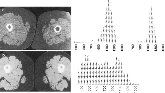
Fig. 26.2
Two examples of abnormal bone demonstrated by CT. (a) Compromised bone geometry at the mid shaft of the femur in a 14-year-old boy 2 months after completion of casting for an injury. The left (injured) leg has a thinned cortex but normal bone density (1,135 ± 115 mg/cm3 K2HPO4) compared with the contralateral leg (1,100 ± 141 mg/cm3 K2HPO4), as indicated by the density histograms on the right of the figure. (b) Compromised material properties at the mid shaft of a 3-year-old boy with familial hypophosphatemic rickets. Bone density (619 ± 366 mg/cm3 K2HPO4) is lower than normal and broadly distributed, while bone geometry is enhanced by increased cortical thickness (Images reprinted from Kovanlikaya et al. [48])
Imaging is used to assess bone microarchitecture. High-resolution imaging can show cortical porosity, trabecular number, trabecular thickness, trabecular separation, and bone volume fraction. These architectural or morphometric properties are analogous to traditional histomorphometric measures. A number of noninvasive imaging techniques can assess and quantify bone properties. The most commonly used techniques include dual-energy x-ray absorptiometry (DXA), quantitative computed tomography (QCT), peripheral quantitative computed tomography (pQCT), magnetic resonance imaging (MRI), and quantitative ultrasound (QUS). The following sections describe these techniques.
2 Dual-Energy X-ray Absorptiometry (DXA)
This technique is most commonly used to assess bone in children and adults, particularly in clinical settings. Advantages of DXA include low cost, widespread availability, ease of use, short scan times, and very low radiation exposure (<4 μSv per scan). Standardized scanning and analysis protocols exist for commonly assessed sites such as the whole body, spine, hip, and forearm. Normative data specific to children are available [10]. However, DXA has several major limitations particularly problematic to measuring bone in growing children and adolescents. These limitations include size dependence of the density measurements due to the two-dimensional (2-D) nature of DXA (Fig. 26.3), inaccuracies associated with nonhomogeneous soft tissue, inclusion of posterior elements in anterior-posterior imaging of the spine, and discrepancies that occur when using different densitometers.
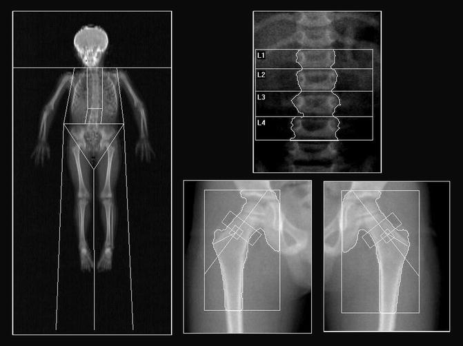
Fig. 26.3
DXA projection images of the whole body, spine, and hips from a healthy 6-year-old boy
DXA measurements of bone rely on the difference in attenuation between high- and low-energy x-ray beams as they pass through soft tissue and bone. The low-energy beam is attenuated more than the high-energy beam in both soft tissue and bone, but the differential is much greater in bone. Subtracting soft tissue attenuation from regions not containing bone yields bone attenuation. Attenuation can then be converted to mass and density by internal phantom calibration.
The resulting measurements provide estimates of bone mineral content (BMC, measured in grams), bone mineral density (BMD, measured in g/cm2), and bone area (BA, measured in cm2). Bone area is the projected area of the bone in a plane perpendicular to the x-ray beams. Bone mineral density is calculated as BMD = BMC/BA. Since BMD is determined using an area rather than a volume, it is referred to as areal BMD (aBMD) to emphasize that it is not a true volumetric density. DXA aBMD can explain approximately 70 % of the variance in bone strength and is a significant predictor of fracture risk in adults [1]. DXA measures may also predict fractures in children and adolescents [11, 12]. Clinical interpretation of DXA results is complex because the World Health Organization (WHO) definition of osteoporosis based on T-scores does not apply to children. Rather, the International Society for Clinical Densitometry (ISCD) recommends the use of Z-scores, with Z-scores of less than −2 considered low for chronological age. In addition, height adjustment is recommended for children with linear growth disturbances or delay in maturation; however, there is no consensus on the method of adjustment.
For populations that commonly present with skeletal deformities, joint contractures, or indwelling hardware, DXA scanning of the lateral distal femur (LDF) is useful. This approach was first developed for use in children with cerebral palsy; the existing protocols were inappropriate for these patients due to their inability to be properly positioned and/or the presence of metal implants at the spine and hips [13]. The method is now used in other pediatric patient populations including children with spina bifida, muscular dystrophy, osteogenesis imperfecta, juvenile arthritis, and other diagnoses [14]. Generally, LDF scanning is feasible in patients for whom standard scans cannot be obtained. In a review of pediatric DXA examinations performed on orthopedic patients, only LDF scans could be obtained in 21 % of children. Hip, spine, and whole body assessments could not be performed in these patients due to contractures or metal instrumentation [15]. Pediatric normative data are available for the LDF scan [16], facilitating estimation of Z-scores and interpretation of the results.
Despite its widespread use, DXA has several major limitations that particularly affect bone measurements in children and adolescents. First, because it is a two-dimensional projection technique, DXA cannot account for the dimensions of the bone in the direction of the x-ray beams. Consequently, larger bones produce higher aBMD measurements even if they do not have higher volumetric density. Various corrections have been proposed to account for this size bias. Unfortunately, these corrections do not work as well in children as in adults, probably because of the osseous changes that occur during growth [17]. To account for the size dependence of DXA, the ISCD recommends that, in addition to chronological age, a measure of growth, such as height or height-age (the age at which a child’s height is the median height-for-age), be taken into account when comparing an individual child to reference data. However, this usually does not completely remove age or height bias [18]. Height-for-age percentiles or Z-scores may provide the best adjustment [18].
The second major limitation of DXA is that it assumes that soft tissue adjacent to bone and soft tissue overlying bone has the same attenuation. Because fat has significantly lower attenuation than other soft tissues, which are considered “lean,” the assumption of homogeneous soft tissue attenuation breaks down when the soft tissue overlying and adjacent to bone contain different proportions of fat. The resulting errors in aBMD can be up to 15 % in adults [19] and 18 % in adolescents, with an average error of 7 % in a large cohort of adolescents and young adults ages 16–25 years [20]. Errors due to soft tissue artifacts may be particularly problematic in overweight or obese individuals and in those who undergo large changes in weight and body composition [21].
A third major limitation of DXA is inclusion of the posterior elements in anterior-posterior imaging of the lumbar spine. Since DXA is a projection technique, the bone measured by DXA includes all bone along the beam path. This includes the cortical and cancellous compartments of the vertebral body, as well as the posterior elements. Although the posterior elements contribute little to vertebral fracture resistance, they add a significant volume of cortical bone, greatly increasing the BMC and aBMD measured by DXA. In fact, the posterior elements contribute approximately half of the total vertebral BMC in children [22]. The percentage of BMC contributed by the posterior elements increases during development but stabilizes after sexual maturity [22]. Therefore, the posterior elements should be considered when measuring DXA aBMD of the lumbar spine in growing children. They are of less concern in older adolescents and young adults.
Finally, DXA measurements are repeatable when acquired on the same machine using the same software but may differ when with different densitometers or software. Discrepancy occurs when manufacturers implement the basic DXA concepts differently. To account for these differences, “universal” measures have been proposed [23]. Unfortunately, these methods have not been widely adopted and are seldom practiced. However, despite its lack of accuracy, DXA is reasonably precise. The short-term in vivo precision of DXA measurements is 0.8–2.5 % in children and 1.5–2.5 % in infants [24, 25]. For longitudinal evaluations, patients should be measured on the same densitometer using the same software. However, care should be exercised in interpreting results since measurements may be influenced by bone morphology or growth.
3 Quantitative Computed Tomography (QCT)
QCT is a three-dimensional imaging technique that allows for segmentation of cortical and trabecular bone regions and separate assessments of bone density, size, and geometry. Unlike DXA, QCT measurements are largely unaffected by soft tissue artifacts. However, QCT is expensive and uses ionizing radiation. QCT assessments of bone mass are mostly used in research but are sometimes performed clinically.
QCT bone measurements are obtained with a standard clinical computed tomography (CT) scanner. X-rays pass through the body in different directions, usually in a spiral or helical pattern, and attenuation is measured for each x-ray transmission. Since each voxel in the region of interest is traversed by multiple x-ray beams traveling in different directions, the data set can be resolved to determine an attenuation value (CT number) for each voxel. The attenuation values are expressed in terms of Hounsfield units (HU), calibrated so water has a value of 0. Cancellous and cortical bones range from 400 to 3,000 HU; fat and air have negative values. In QCT imaging, a bone mineral reference phantom is placed under the patient during scanning (Fig. 26.4). The phantom enables conversion of HU to a hydroxyapatite equivalent density measured in mg/cm3.
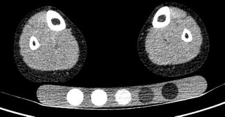
Fig. 26.4
QCT image of a healthy 11-year-old boy at the mid-tibia level showing bone mineral reference phantom. The phantom allows for quantification of hydroxyapatite equivalent volumetric bone mineral density
QCT measurements of cortical bone density represent the bone’s material density as long as the cortex is sufficiently thick to avoid volume averaging errors (>2.0–2.5 mm) [26]. The CT value of cortical bone depends primarily on the calcified bone volume fraction because bone mineral has a very high attenuation coefficient.
In cancellous bone, the trabeculae are small relative to the size of the voxel. QCT values therefore reflect not only the amount of mineralized bone and osteoid but also the amount of marrow in each voxel [27]. On average, the CT values of cortical bone are eight times higher than those of cancellous bone. This reflects the porous nature of cancellous bone, not a difference in bone material.
In addition to measures of cortical and cancellous bone density, QCT can be used to obtain measures of three-dimensional bone geometry. Cross-sectional area and volume are often measured, along with cortical bone area for diaphyseal sites. The cross-sectional images can also determine structural parameters that reflect bone stiffness and strength such as moments of inertia, section modulus, and stress-strain index. The coefficients of variation for QCT measurements of bone density and geometry are between 1 and 2 %.
QCT measures of volumetric cancellous bone density in the lumbar vertebrae increase primarily during puberty and peak by late adolescence (Fig. 26.5) indicating that puberty is the critical period for building cancellous bone mass. In contrast, long bones increase in diameter throughout life due to the ongoing processes of periosteal apposition and endosteal resorption. This difference in growth patterns may contribute to the increasing susceptibility of cancellous sites such as the hip and spine to fracture with aging.
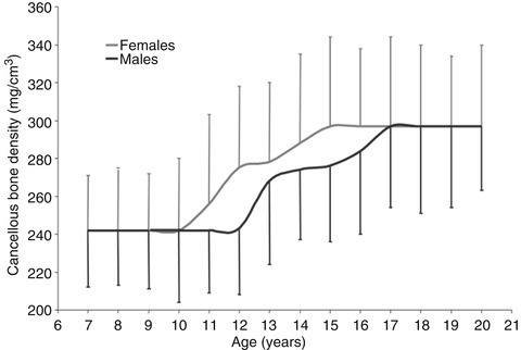
Fig. 26.5
Changes in vertebral cancellous bone density during growth. Density does not begin increasing until approximately age 10 years in females and age 12 years in males. Density reaches its peak by age 15 years in females and age 17 years in males (Reprinted with permission from Gilsanz et al. [49])
Most clinical assessments of bone using QCT evaluate a localized region such as a slice through the middle of the vertebral body or femur (Fig. 26.6). Volumetric QCT can be performed but is not widely used due to radiation concerns. Clinical studies in adults have used volumetric QCT to examine the hip and spine [28], but this has not been done in children. However, volumetric QCT has been used in children at peripheral sites such as the tibia and radius (Fig. 26.7) where relatively low radiation exposure is possible.
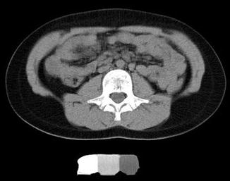
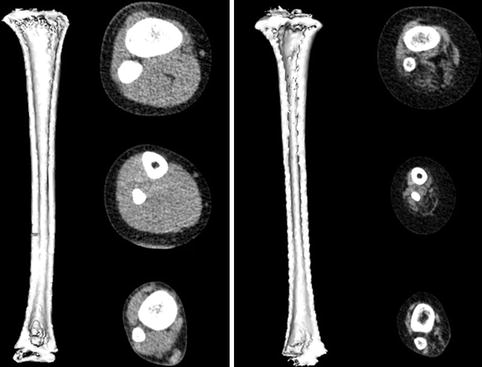
Fig. 26.6
QCT image of the L3 vertebra in an ambulatory 10-year-old girl with diplegic cerebral palsy
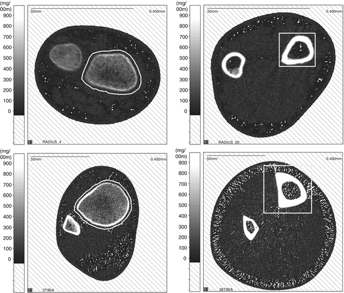
Fig. 26.7
Volumetric QCT images of the tibia in a healthy 6-year-old boy (left) and a 6-year-old boy with lumbar level myelomeningocele (right). The child with myelomeningocele has a smaller bone with thinner cortices. Muscle volume and density are also greatly reduced in the child with myelomeningocele
The main advantage of volumetric QCT is that it allows for assessment of entire structures. Examining a single slice may miss the weakest and most vulnerable section of the bone. In addition, certain regions such as the metaphyses of long bones are not uniform, making measurement at a single site problematic. In the proximal tibial metaphysis, for example, cancellous bone density changes by an average of 7 mg/cm3 or 17 % for each millimeter along the length of the metaphysis [29] (Fig. 26.8). A small change in slice location therefore results in a large change in measured density. In longitudinal studies, even if the site of measurement can be replicated exactly, changes in morphology due to growth make it difficult to compare measurements.
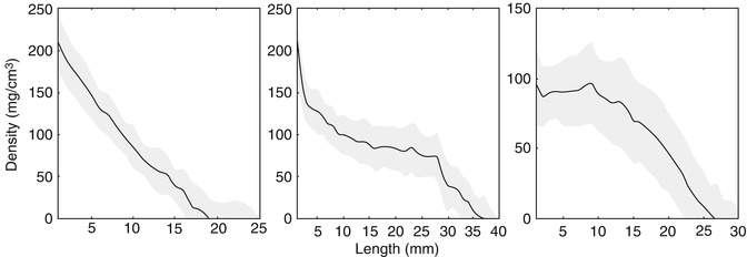
Fig. 26.8
Change in cancellous bone density along the length of the metaphysis in three ambulatory children with cerebral palsy (Reprinted with permission from Lee et al. [29])
Radiation exposure is QCT’s main drawback. For QCT measurements of bone, the radiation exposure can be as low as 1.5 mSv localized to the region of interest, with a total body equivalent dose of approximately 40–90 μSv including the localizer images [30, 31]. This is similar to the amount of radiation exposure that occurs during a round-trip flight across North America [30, 31] and much lower than the radiation associated with other CT imaging procedures.
4 Peripheral Quantitative Computed Tomography (pQCT)
PQCT is similar to QCT except that it uses scanners specifically designed to deliver doses of radiation that are generally less than 5 mSv. This is comparable to DXA and much lower than conventional CT [32]. In addition to lower radiation exposure, pQCT scanners are smaller, more portable, and less expensive. The main limitation of pQCT is that it is only used for peripheral sites. PQCT is most commonly used to measure the distal radius and tibia (Fig. 26.9), although some scanners can image the pediatric femur and humerus. The primary measurements obtained are the same as for QCT, i.e., the density and cross-sectional properties of trabecular and cortical bone.