Brain CT Perfusion Imaging: Cerebral Ischemia

Christopher D. d’Esterre, BMSc, PhD

Mohammed Almekhlafi, MD

Bijoy K. Menon, MD,

Mayank Goyal, MD, FRCPC

▪ Introduction

Stroke is caused by variable disturbances in blood flow to intracranial structures due to lack of blood supply (ischemia) or leakage of blood from vessels (hemorrhage). Accordingly, these cerebrovascular accidents have distinct etiologies: the former caused by thromboembolism or systemic hypoperfusion leading to local or global cerebral ischemia, respectively, and the latter caused by a rupture of weakened vascular walls within or around brain tissue. In the past 40 years, the use of medical imaging to distinguish stroke subtypes has become a mainstay at almost all medical institutions, revolutionizing acute diagnosis and treatment, as well as improving prediction of long-term patient outcome. For both clinical and experimental stroke, details of the anatomical structure and function of the brain are currently possible with multimodal imaging. Computed tomography (CT), magnetic resonance imaging (MRI), and positron emission tomography (PET) have helped guide acute stroke triage and advanced our knowledge of pathophysiologic mechanisms guiding stroke treatment strategies. However, PET imaging in acute stroke remains limited to research studies in academic centers due to its cost and logistical/technical complexities. PET tracers and scanners will continue to evolve, but it is unlikely that PET will see widespread clinical use for acute stroke patients in the near future. MRI is more readily available in the setting of acute stroke and does not require a radioactive substance to be injected. Further, most sequences, unlike CT, are able to cover both supra- and infratentorial brain regions, allowing a more robust diagnostic imaging window and increased prognostic sensitivity. In terms of patient throughput, individuals who are claustrophobic or have metal implants and pacemakers are excluded from MRI. Further, MRI scanners have limited availability, primarily accessible at large city hospitals or academic centers. CT imaging is a diagnostic tool that is widely available, relatively inexpensive compared to its acute stroke counterpart, MRI, noninvasive, and fast. The acute CT imaging stroke series generally consists of a noncontrast CT (NCCT), followed by multiphase CT angiography (mCTA), for patients with stroke symptoms; however, critical information about the underlying pathophysiology may be overlooked. In a few added minutes, further assessment of cerebral hemodynamics with CT perfusion (CTP) can give insight into early ischemic changes (EICs), tissue states, and blood-brain barrier (BBB) disturbances, unseen on NCCT/CTA. Moreover, due to optimized scanning protocols, the added radiation dose is minimized.

Herein, we discuss CTP data acquisition, mathematical models, limitations and diagnostic caveats, and the potential of CTP to improve acute stroke management related to cerebral ischemia.

▪ CT Perfusion Acquisition

CTP imaging depends on the speed of multidetector row (from 16 to 320 rows) scanners to follow the entry and exit of radiographic dye through an imaging volume or “slab of tissue.” For each CTP study, 35 to 45 mL of a nonionic iodinated contrast agent, at a concentration of 300 to 370 mg iodine/mL, is power injected into an arm vein (typically the cephalic vein); injection rates can vary from 4 to 6 mL/s, followed by a saline flush of 20 to 40 mL at identical rates. The faster the injection rate, the “tighter” the contrast bolus, which results in a sharper, narrower, and higher peak in the time-attenuation curve (TAC). However, these fast injection features require an image acquisition of one image approximately every 2.5 seconds to characterize the peak of the arterial curve accurately, which is essential for the accurate calculation of CTP hemodynamic parameters. Imaging is performed at a constant milliampere-second (100 to 200 mAs) and a kilovoltage (kV) of 80; this kV setting generates photons with mean energy close to the k-edge of iodine, maximizing the photoelectric effect, and subsequent contrast visibility. Axial shuttle (step and shoot) mode is used to cover 8-cm section of the brain including the intracranial ICA at 5-mm slice thickness. Data acquisition generally starts 4 to 6 seconds after injection and before the contrast reaches the tissue of interest to measure the baseline of the TAC, which is subtracted off the entire curve as the first postprocessing step. For perfusion studies without the need to investigate BBB integrity, an acquisition time interval of 70 to 90 seconds is recommended.¹ If measurement of BBB permeability is also required along with perfusion measurements, a two-phase acquisition is more appropriate, in which the first phase lasting 45 to 50 seconds at a rapid imaging rate of one image every 1 to 3 seconds is followed by a slower second phase of one image every 10 to 15 seconds for another 2 minutes.²

▪ CTP Raw Data Processing

Depending on the clinical symptoms, the imaged volume is selected at the level of the basal ganglia, which includes posterior, anterior, and middle cerebral arteries. CTP describes hemodynamics within
the entire vasculature including large arteries, arterioles, capillary beds, venules, and veins. As an intravascular contrast bolus passes through a mass of brain tissue, the signal intensity of each voxel within a CT image will change over time. The intensity of the CT image, expressed in Hounsfield units (HU), is linearly proportional to the efficiency with which ionization radiation, in the form of x-rays, is attenuated. With current CTP software, processing of these hemodynamic functional maps is practically automated. The operator needs only to select an arterial input function (AIF) and a venous output function (VOF). The AIF is selected from within a large artery (usually the basilar or internal carotid artery), preferably at a location along the artery where it is orthogonal to the scan plane to limit partial volume averaging (PVA)—this “dilution” effect will become apparent when comparing the peak enhancement (increase of attenuation above baseline) of arteries of different sizes. The VOF is selected from a large vein, usually the superior sagittal sinus, to minimize the effect of PVA on its accurate measurement. As such, the underestimation of the AIF from PVA can be corrected by normalizing the area of the AIF with that of the VOF.³

Perfusion Parameters

For each pixel, its TAC is used to quantify several perfusion parameters: cerebral blood flow (CBF), the volume rate of blood moving though the mass of tissue (mL/min/100 g); cerebral blood volume (CBV), the total volume of moving blood in the mass of tissue (mL/100 g); the time to peak (TTP) of the pixel TAC corrected for the dispersion in the artery TAC (T_o) or the time to maximum of the tissue residue function; and a new parameter, which is discussed in detail in later sections, the permeability surface area product (PS) of the BBB (mL/min/100 g) (Fig. 13.1). Calculation of these parameters is described below. Another perfusion parameter useful for acute ischemic evaluation is the TTP (T_max) of the impulse residue function (IRF). This is different from the TTP of the tissue TAC. The latter is confounded by the TTP of the AIF and therefore reflects not only the local hemodynamics of the tissue but also that of the central (systemic) circulation. The T_max of the IRF is the summation of the delay between the arrival times of contrast at the artery and tissue region as well as mean transit time (MTT) of the local vasculature. The delay reflects the adequacy of collateral circulation to the region, while MTT is inversely related to the perfusion pressure in the local vasculature.⁴ Unlike the calculation of absolute CBF or CBV, the calculation of T_max is independent of the calibration between the AIF and tissue TAC; as such, it is increasingly being used in perfusion-weighted DCE-MR for the determination of the tissue at risk in stroke.⁵,⁶ However, calculation of T_max requires deconvolution of the tissue TAC, which is more complex than determining the TTP of the tissue TAC. It has been shown recently by comparison with PET that T_max maps did not perform better than the more easy-to-obtain nondeconvolved TTP maps in identifying ischemic penumbra.⁷ Moreover, the T_max definition can be different between vendors due to IRF assumptions and modeling, especially between MRP and CTP modalities.⁸

Figure 13-1. Sample cerebral blood flow (CBF), cerebral blood volume (CBV), time-to-peak of tissue-residue-function (T_max), and PS CTP functional maps for the patient with ischemic stroke. Color-coded functional maps of CBF, CBV, T_max, and permeability surface area product (PS) calculated using CT perfusion software (GE Healthcare). CBF is expressed in units of mL/100 g/min, CBV in mL/100 g, T_max in seconds, and PS in mL/100 g/min.

CTP Mathematical Models

Deconvolution- and non-deconvolution-based models are used to calculate perfusion parameters. Although physiologically more appropriate, deconvolution models involve complex algorithms and require more time for the calculation, whereas the simplicity of nondeconvolution models stems from their simplified assumptions about hemodynamics in the brain that may not hold true in general.

Deconvolution Approach

Deconvolution methods correct for the inability to deliver a contrast bolus directly into the supplying artery of a tissue of interest— the bolus introduced at a peripheral vein undergoes “delay” and “dispersion” prior to its arrival at the artery to become the AIF or the TAC of the artery. Deconvolution corrects for this by calculating an IRF, which depends on the concept of convolution, and simulates the tissue TAC, which would be obtained under the ideal injection condition. For brain imaging, the governing convolution equation for the tissue TAC is as follows:

where ⊗ is the convolution operator; C_a(t) and Q(t) are the artery and the tissue TAC, respectively; and CBF·R(t) is the CBFscaled IRF.⁹ The height and area of the flow-scaled IRF are CBF and CBV, respectively, and MTT is the ratio of CBV to CBF as required
by the central volume principle.¹⁰ In a CTP study, the arterial and tissue TAC, C_a(t) and Q(t), are measured, the problem concerns the deconvolution of Q(t) to calculate CBF·R(t). Convolution of the AIF with flow-scaled IRF gives a unique (unambiguous) tissue TAC because it is the summation of different versions of the known CBF·IRF with each version being the original CBF·IRF shifted in time and scaled with the AIF.⁸ On the other hand, deconvolution estimates the unknown CBF R(t), such that its convolution with the arterial TAC would approximate (fit) the tissue TAC as closely as possible. Therefore, deconvolution solutions are ambiguous, as there are many CBF·R(t)s, which after convolution with C_a(t) are able to give equally good fits to the tissue TAC. Furthermore, many of these CBF R(t)s can have shapes that are not consistent with the physiologic behavior of an IRF, for instance, oscillating between positive and negative values, due to noise in either the arterial or tissue TAC.¹¹ These effects can be mitigated with noise suppression in the deconvolution algorithm to obtain a physiologically more plausible IRF as shown in Figure 13.2, from which more accurate perfusion parameters can be estimated as discussed above.¹²

Another hemodynamic parameter, new to stroke imaging, is the permeability surface area product (PS). PS is the product of permeability and the total surface area of perfused capillary endothelium within an unit mass of tissue and is the total diffusional flux across all perfused capillaries.¹³ Currently available CTP software uses either compartmental or the Johnson-Wilson (J-W) model to describe the distribution of contrast in brain tissue. ¹³,¹⁴ and ¹⁵ Compartmental models can only measure PS and CBV, not CBF, because contrast distribution in the brain is determined only by diffusion when PS is much smaller than CBF.¹³ The Patlak approach simplifies the compartmental model further by assuming the absence of contrast agent backflux from the interstitial to the intravascular space (IVS).¹⁶ Under the Patlak assumption, the normalized tissue concentration is linearly related to the normalized time, with the slope and intercept of the linear regression line being equal to PS and CBV, respectively.¹⁶ However, the assumption of no backflux of contrast from the interstitial to IVS in the Patlak model is physiologically not possible for a leaky BBB.² In theory, use of the Patlak model can lead to an underestimation of PS.² The J-W model does not invoke the Patlak assumption of no tracer backflux, and unlike compartmental models, it allows CBF to be estimated together with CBV and PS.¹³ The J-W model divides the brain into two principal spaces: the IVS and the extravascular space (EVS), separated by a capillary endothelium of variable PS, therefore applicable to both permeable and impermeable BBBs. Assumptions for the J-W model include bidirectional diffusion of contrast agent between the EVS and IVS and an axial contrast concentration gradient in the capillaries, and contrast concentration is assumed to have a homogeneous spatial distribution within EVS.¹⁷,¹⁸ The adiabatic approximation to the J-W model assumes that the contrast concentration in the EVS is changing slowly relative to the rate of change of concentration in the IVS.¹⁸ Under this approximation, the IRF R(t) can be represented simply as

Figure 13-2. The IRF can be viewed as the fraction of contrast medium that remains in the tissue as time evolves following a bolus injection into the arterial input. Beyond the minimum transit time (the duration of the plateau), the difference of R(t + Δt) and R(t) is the fraction of contrast medium that has a transit time of t. This difference is the height of the strip with a transit time of t. Further, the area of each of the horizontal strips is the product of the transit time and the fraction of contrast medium having that transit time. It follows that the area of all the horizontal strips, that is, the area under the curve (AUC) of R(t), is the MTT. Alternatively, as the Central Volume Principle states that the product of CBF and MTT is CBV, the AUC of CBFR(t) is the CBV.

where T_c is the MTT of blood through the brain and F is CBF, so that CBV is F · T_c according to the central volume principle.³ E is the contrast extraction fraction, and V_c is the contrast agent distribution volume in the EVS. E relates to the PS of the BBB by the following relationship:

If C_a(t) is the AIF to the brain, then the measured brain tissue curve Q(t) can be calculated as the convolution of C_a(t) and R(t):

where ⊗ is the convolution operator, and T₀ is the appearance time of contrast agent in the brain relative to that in the input artery. Equation (4) is valid under the assumption that brain blood flow is constant and Q(t) is linear with respect to C_a(t). With Q(t) and C_a(t) having been measured in a CTP study, CT Perfusion 4D (GE Healthcare, Waukesha, WI) estimates the parameters CBF, CBV, T_c, PS, and T₀ of each voxel by iteratively changing their values until an optimum fit to Q(t) is achieved by means of Eqs. (2),(4).

Nondeconvolution Approach

Similar to the deconvolution models, nondeconvolution (model independent) approaches are based on the Fick principle of conservation of mass.¹⁹ The maximal slope method calculates CBF as the ratio of the maximum initial slope of the tissue TAC to the peak height of the arterial TAC.³,¹⁹ Although conceptually simple, the assumption of having no venous outflow at the time of maximum initial slope is rarely true; therefore, a global CBF underestimation is possible with this method. However, when compared to deconvolution methods, the maximum slope model provides similar functional map quality and quantitative values for acute infarct delineation, guiding thrombolysis treatment.²⁰

Acquisition and Processing Caveats and Concerns

Spatial Coverage and Patient Motion

The volume of brain tissue that can be imaged in one CTP acquisition is limited in the craniocaudal direction (z-axis for all scanners) by the number of detector rows in a CT scanner to between 4 and 16 cm with current models of scanners. Coverage in this direction can be doubled (to include two adjacent sections of the brain) using shuttle mode or two separate boluses.²¹,²² The shuttle technique can have two variations, step and shoot (axial shuttle) or continuous table translation (helical shuttle) between the two sections. Axial shuttle mode generally has less motion artifact than helical shuttle mode as images are acquired with the patient table (brain) stationary during the former. Also, the image interval of all slices in axial shuttle mode is uniform (2 to 3 seconds), while the helical shuttle mode is nonuniform for the cranial and caudal slices—the image intervals for slices in the centre of the two-section volume will be roughly uniform at 2 to 3 seconds, and those for the more cranial and caudal slices of that volume can vary from 1-2 to 4-5 seconds. The two injections technique requires double the dosage of iodinated contrast increasing the risk of affecting kidney function. However, a recent multicenter study has shown that the incidence of contrast-induced nephrotoxicity was low approximately 2.6% among at-risk patients undergoing contrast-enhanced CT scans in a “real-world” clinical setting, where guideline-recommended strategies for contrast induced nephrotoxicity prevention may not be consistently followed.²³

Patient-related motion is a major source of image artifact in an acute stroke CTP study. During acquisition, the patient’s head is normally held with a plastic head holder mounted to the scanner table to minimize the head movement. The holder can reduce but not completely eliminate head movement in some cases. Figure 13.3 shows how the arterial and tissue TACs can be affected by movement in the x—y plane, despite the use of such a head holder. Temporal registration and/or removal of images can correct for x—y plane patient motion. With z-axis motion, removal of images is more difficult than x—y motion as slice locations change during the cine acquisition.

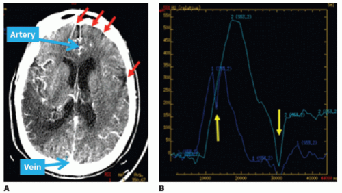Figure 13-3. A: Movement of the patient’s head during acquisition caused significant artifacts (red arrows) in the DCE CT images. B: The arterial and venous TACs were significantly affected and exhibited large fluctuations (yellow arrows).

Ionizing Radiation

Although a 60- to 70-second imaging protocol is sufficient for a perfusion-only study, acquisitions of 90- to 180-second durations have been advocated for combined perfusion and BBB permeability studies.²,²⁴,²⁵ and ²⁶ To minimize radiation exposure from the lengthened scan time required for blood-brain permeability measurement, temporal sampling is decreased to one image every 10 to 15 seconds after the first phase as has been discussed above in section (1).²⁵ The total effective dose from a multimodal CT stroke study, for a 64-row detector CT, is approximately 7 mSv—this is double the average annual background radiation.²⁷ Radiation dose reduction strategies, such as the adaptive statistical iterative reconstruction, can maintain image quality while reducing effective dose by greater than 25%.²⁸ Also, radiation dose could be reduced by two-thirds, without compromising the accuracy of the CTP functional maps, by increasing the sampling interval from 1 to 3 seconds in the first phase of a CTP study.²¹

Delay and Dispersion of the AIF

As described in section (1), an AIF measured from a large artery is required in the deconvolution of the tissue TAC to calculate tissue perfusion. Because of time causality, deconvolution formulated as the inversion of a system of linear equations using singular value decomposition (SVD) works properly only if the tissue TAC lags behind the AIF in time, that is, the contrast arrival time of the tissue TAC is later than that of the AIF (positive delay). If there is negative delay between the AIF and tissue TAC, standard deconvolution formulation with SVD will overestimate CBF and underestimate MTT.²⁹ The problem with perfusion studies of stroke patients is that both positive and negative delays between the chosen AIF and tissue TAC could occur in the same study. If the AIF is measured from an artery downstream from an occlusion, TAC of normal brain will lead the ipsilateral AIF in time (negative delay) while the TAC of ischemic brain may have the same or delayed contrast arrival time as that of the ipsilateral AIF (positive delay). In this situation, it is important to formulate the deconvolution as inversion of a block-circulant matrix with the SVD technique. It has been shown using simulations that block-circulant deconvolution with SVD produces CBF estimates that are independent of whether the delays between the AIF and tissue TACs are positive or negative.³⁰

Besides using block-circulant deconvolution with SVD to minimize the effects of the negative delays between the ipsilateral AIF and tissue TACs, choosing an AIF from an artery in the contralateral (unaffected) hemisphere could avoid the presence of negative delays. However, the blood supply to an ischemic region is mainly via collateral circulation such that besides delay in arrival times, the AIFs measured in ipsilateral arteries are also dispersed with respect to the AIFs measured in contralateral arteries. The use of a nondispersed contralateral AIF rather than the true dispersed ipsilateral AIF to deconvolve the tissue TAC will underestimate the true blood flow.³¹ It has been proposed that dispersed ipsilateral AIF can be measured by independent component analysis (ICA) of the ischemic region.³¹ ICA is a data-driven technique, which is based on analyzing the time behavior of all TACs in a region and trying to decompose the TACs into linear combinations of a few dominant temporal patterns (independent components). In a perfusion study, a few of the independent components that are similar in their temporal behavior to that expected of AIF in locations that are mostly in arteries are summed together to produce the local AIF. The disadvantages of using ICA to define the local AIF are as follows: first, the choice of which independent components to retain to represent the AIF is arbitrary; second, the spatial mask used to select locations (presumably arteries) from which the chosen independent components are summed to generate the local AIF is also arbitrary. As such, the ICA algorithm for the generation of local AIF has to be validated; so far, no validation studies have been reported.

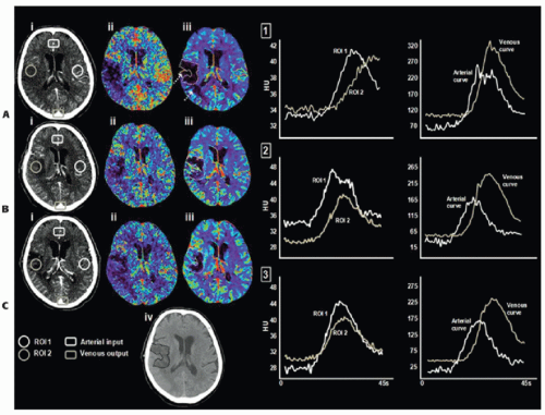Figure 13-4. CTP-derived contrast-enhanced image, CBF (scale 0 to 150 mL/min/100 g) and CBV (scale 0 to 8 mL/100 g) functional maps (i–iii) at admission, 24 hours, and 7 days poststroke onset (A to C). NCCT from 7 days poststroke shows outlined infarct region (iv). Corresponding time-density curves (Hounsfield units versus time) were taken at each time point. Confluent areas outside of superimposed infarct ROI showing CBV lesion overestimation (dashed arrows); at this time, TDC_i truncation is apparent. CBV_I reversibility is observed at 24 hours and 7 days, compared to admission, for this patient.

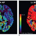
Given the above considerations on the effects of delay and dispersion of the AIF on the estimation of perfusion parameters, it is recommended that the AIF can be chosen from the contralateral (normal) hemisphere as several studies have demonstrated that ipsilateral or contralateral placement of the AIF does not affect calculation of CBF and block-circulant or other delay-insensitive deconvolution algorithms should be used.³²,³³

CTP Data Truncation

For CTP perfusion studies with an acquisition interval limited to 45 to 50 seconds, the TAC of an ischemic region can be truncated, that is, data acquisition terminates before the TAC reaches the washout phase. As CBV is related to the area of the TAC, truncation leads to underestimation of the area and hence CBV of the ischemic region.²² In previous work, the ability of the acute CTP-derived CBV lesion (i.e., CBV close to zero) to predict nonviable ischemic tissue has been demonstrated.³⁴,³⁵ and ³⁶ Most recently, CBV evolution was examined in 13 patients within gray and white matter destined to infarct, as defined by NCCT at 7 days postadmission, as well as overestimation of the infarct core, as defined by the CBV abnormality at admission.³⁷ CBV reversibility out to 7 days postadmission was observed in four patients; however, this reversal was more common in patients with an incomplete washout (truncation) of the tissue TAC at admission and/or 24 hours poststroke ictus (Fig. 13.4). It is important to note that complete wash-in and washout of the AIF and VOF does not mean the ischemic tissue TAC is free of truncation. The area and the ratio of area to
height of the flow-scaled IRF represent CBV and MTT, respectively. Therefore, the truncation artifact will underestimate both parameters. On the contrary, CBF is related to the front slope of the tissue TAC (or equivalently the height of the flow-scaled IRF) and therefore is minimally affected by the truncation artifact. Campbell et al.³⁸ and Kamalian et al.³⁹ both demonstrated the ability of absolute and relative (to contralateral hemisphere) CBF values to better approximate diffusion-weighted imaging (DWI) infarct core, compared to CBV and MTT parameters. In the study by Campbell et al., the CTP data were acquired out to 45 seconds, as such, truncation may have affected the calculation of both CBV and MTT, while the study by Kamalian et al. used an appropriate two-phase acquisition (0.5-second sampling for 40 seconds, a 2-second pause, and eight more images every 3 seconds).

Figure 13-5. Dynamic CT measurement plotted against microsphere measurement of rCBF (mL/min/100 g). r = 0.837, p < 0.001, slope of the regression line was close to unity (0.97 ± 0.03).

Preclinical Validation

Fluorescent microspheres have been used for the past 30 years for validating regional CBF (rCBF) measurement methods.⁴⁰ Cenic et al.¹² validated CTP-derived rCBF measurements, using this ex vivo microsphere technique. Specifically, closely spaced (<1 minute apart) measurements of the deconvolution-based dynamic CTPrCBF and microsphere-based rCBF were determined in a healthy rabbit model.¹² A strong correlation was found between the dynamic CTP-rCBF and the fluorescent microsphere rCBF measurements (Fig. 13.5). The mean rCBF obtained from dynamic CTP and microsphere techniques for n = 39 measurements was 73.3 ± 31.5 mL/min/100 g and 74.3 ± 31.6 mL/min/100 g, respectively. This correlation compares well with the findings from others who have validated their dynamic CT and stable xenon-CT techniques with microsphere measurements.⁴¹,⁴² CBV has yet to be validated in the brain.

▪ CTP Applications in Ischemic Stroke

The Use of CT Perfusion to Define Acute Tissue States in Acute Ischemic Stroke

The understanding of the ischemic cascade brought forth distinct definitions of tissue status during hyperacute cerebral ischemia. Within the most hypoperfused territory, called the ischemic or infarct core, neurons are irreversibly damaged, even upon reperfusion, and are no longer viable.⁴³ Across species, the threshold for irreversible neuronal death has been identified as a CBF value of approximately 8 to 10 mL/min/100 g.⁴⁴,⁴⁵,⁴⁶,⁴⁷ and ⁴⁸ The infarct core, consisting of apoptotic/necrotic tissue, is surrounded by a variably sized tissue region with blood flow above the threshold to induce immediate infarction—the ischemic penumbra. The original definition of this tissue state is based on the absence of electroencephalography signals and sensory evoked potentials with maintenance of membrane pump function and ionic gradients retained at near-normal levels.⁴⁹,⁵⁰ Due to this electrical silence, clinical symptoms relating to the affected tissue region are apparent; therefore, it is impossible to discern the amount of viable penumbral tissue based on clinical symptoms alone. The survival of penumbral tissue on the border zone of infarction is largely dependent on leptomeningeal collateral supply, as well the severity of periinfarct depolarization.⁵¹ If blood flow is not restored promptly, the viable ischemic penumbra invariably progresses to infarction; however, with reperfusion in a timely manner, this tissue will fully recover, along with clinical function. This timecritical viability of the ischemic penumbra introduced the “time is brain” paradigm.⁵² Depending on the technique for measuring CBF, the upper threshold for electrical silence and neuronal dysfunction occurs at a CBF of 22 to 25 mL/min/100 g.⁴⁷ The duration of ischemia will determine tissue fate below this threshold.⁵³ A third tissue state is described as having a CBF above the upper threshold for neuronal dysfunction, but lower than normal CBF values, called benign oligemia. Regardless of the duration of ischemia, this tissue does not progress to infarction and maintains normal cellular function, in spite of appreciated hypoperfusion and absence of reperfusion.⁵⁴

Only gold members can continue reading. Log In or Register to continue