Cell Survival Curves

▪ REPRODUCTIVE INTEGRITY

A cell survival curve describes the relationship between the radiation dose and the proportion of cells that survive. What is meant by “survival”? Cell survival, or its converse, cell death, may mean different things in different contexts; therefore, a precise definition is essential. For differentiated cells that do not proliferate, such as nerve, muscle, or secretory cells, death can be defined as the loss of a specific function. For proliferating cells, such as stem cells in the hematopoietic system or the intestinal epithelium, loss of the capacity for sustained proliferation— that is, loss of reproductive integrity—is an appropriate definition. This is sometimes called reproductive death. This is certainly the end point measured with cells cultured in vitro.

This definition reflects a narrow view of radiobiology. A cell may still be physically present and apparently intact, may be able to make proteins or synthesize DNA, and may even be able to struggle through one or two mitoses; but if it has lost the capacity to divide indefinitely and produce a large number of progeny, it is by definition dead; it has not survived. A survivor that has retained its reproductive integrity and is able to proliferate indefinitely to produce a large clone or colony is said to be clonogenic.

This definition is generally relevant to the radiobiology of whole animals and plants and their tissues. It has particular relevance to the radiotherapy of tumors. For a tumor to be eradicated, it is only necessary that cells be “killed” in the sense that they are rendered unable to divide and cause further growth and spread of the malignancy. Cells may die by different mechanisms, as is described here subsequently. For most cells, death while attempting to divide, that is, mitotic death, is the dominant mechanism following irradiation. For some cells, programmed cell death, or apoptosis, is important. Whatever the mechanism, the outcome is the same: The cell loses its ability to proliferate indefinitely, that is, its reproductive integrity.

In general, a dose of 100 Gy is necessary to destroy cell function in nonproliferating systems. By contrast, the mean lethal dose for loss of proliferative capacity is usually less than 2 Gy.

▪ THE IN VITRO SURVIVAL CURVE

The capability of a single cell to grow into a large colony that can be seen easily with the naked eye is a convenient proof that it has retained its reproductive integrity. The loss of this ability as a function of radiation dose is described by the dose-survival curve.

With modern techniques of tissue culture, it is possible to take a specimen from a tumor or from many normal regenerative tissues, chop it into small pieces, and prepare a single-cell suspension by the use of the enzyme trypsin, which dissolves and loosens the cell membrane. If these cells are seeded into a culture dish, covered with an appropriate complex growth medium, and maintained at 37° C under aseptic conditions, they attach to the surface, grow, and divide.

In practice, most fresh explants grow well for a few weeks but subsequently peter out and die. A few pass through a crisis and continue to grow for many years. Every few days, the culture must be “farmed”: The cells are removed from the surface with trypsin, most of the cells are discarded, and the culture flask is reseeded with a small number of cells, which quickly repopulate the culture flask. These are called established cell lines; they have been used extensively in experimental cellular radiobiology.

Survival curves are so basic to an understanding of much of radiobiology that it is worth going through the steps involved in a typical experiment using an established cell line in culture.

Cells from an actively growing stock culture are prepared into a suspension by the use of trypsin, which causes the cells to round up and detach from the surface of the culture vessel. The number of cells per unit volume of this suspension is counted in a hemocytometer or with an electronic counter. In this way, for example, 100 individual cells may be seeded into a dish; if this dish is incubated for 1 to 2 weeks, each single cell divides many times and forms a colony that is easily visible with the naked eye, especially if it is fixed and stained (Fig. 3.1). All cells making up each colony are the progeny of a single ancestor. For a nominal 100 cells seeded into the dish, the number of colonies counted may be expected to be in the range of 50 to 90. Ideally, it should be 100, but it seldom is for various reasons, including suboptimal growth medium, errors and uncertainties in counting the cell suspension, and the trauma of trypsinization and handling. The term plating efficiency indicates the percentage of cells seeded that grow into colonies. The plating efficiency is given by the formula

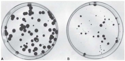FIGURE 3.1 Colonies obtained with Chinese hamster cells cultured in vitro. A: In this unirradiated control dish, 100 cells were seeded and allowed to grow for 7 days before being stained. There are 70 colonies; therefore, the plating efficiency is 70/100 or 70%. B: Two thousand cells were seeded and then exposed to 8 Gy of x-rays. There are 32 colonies on the dish. Thus, Surviving fraction = Colonies counted/[Cells seeded × (PE/100)] = 32/(2,000 × 0.7) = 0.023

There are 70 colonies on the control dish in Figure 3.1A; therefore, the plating efficiency is 70%. If a parallel dish is seeded with cells, exposed to a dose of 8 Gy of x-rays, and incubated for 1 to 2 weeks before being fixed and stained, then the following may be observed: (1) Some of the seeded single cells are still single and have
not divided, and in some instances the cells show evidence of nuclear deterioration as they die an apoptotic death; (2) some cells have managed to complete one or two divisions to form a tiny abortive colony; and (3) some cells have grown into large colonies that differ little from the unirradiated controls, although they may vary more in size. These cells are said to have survived because they have retained their reproductive integrity.

In the example shown in Figure 3.1B, 2,000 cells had been seeded into the dish exposed to 8 Gy. Because the plating efficiency is 70%, 1,400 of the 2,000 cells plated would have grown into colonies if the dish had not been irradiated. In fact, there are only 32 colonies on the dish; the fraction of cells surviving the dose of x-rays is thus

In general, the surviving fraction is given by

This process is repeated so that estimates of survival are obtained for a range of doses. The number of cells seeded per dish is adjusted so that a countable number of colonies results: Too few reduces statistical significance; too many cannot be counted accurately because they tend to merge into one another. The technique is illustrated in Figure 3.2. This technique, and the survival curve that results, does not distinguish the mode of cell death, that is, whether the cells died mitotic or apoptotic deaths.

▪ THE SHAPE OF THE SURVIVAL CURVE

Survival curves for mammalian cells usually are presented in the form shown in Figure 3.3, with dose plotted on a linear scale and surviving fraction on a logarithmic scale. Qualitatively, the shape of the survival curve can be described in relatively simple terms. At “low doses” for sparsely ionizing (low-linear energy transfer [LET]) radiations, such as x-rays, the survival curve starts out straight on the log-linear plot with a finite initial slope; that is, the surviving fraction is an exponential function of dose. At higher doses, the curve bends. This bending or curving region extends over a dose range of a few grays. At very high doses, the survival curve often tends to straighten again; the surviving fraction returns to being an exponential function of dose. In general, this does not occur until doses in excess of those used as daily fractions in radiotherapy have been reached.

By contrast, for densely ionizing (high-LET) radiations, such as α-particles or low-energy neutrons, the cell survival curve is a straight line from the origin; that is, survival approximates to an exponential function of dose (see Fig. 3.3).

Although it is a simple matter to qualitatively describe the shape of the cell survival curve, finding an explanation of the biologic observations in terms of biophysical events is another matter. Many biophysical models and theories have been proposed to account for the shape of the mammalian cell survival curve. Almost all can be used to deduce a curve shape that is consistent with experimental data, but it is never possible to choose among different models or theories based on goodness of fit to experimental data. The biologic data are not sufficiently precise, nor are the predictive theoretic curves sufficiently different, for this to be possible.

Two descriptions of the shape of survival curves are discussed briefly with a minimum of mathematics (see Fig. 3.3). First, the multitarget model that was widely used for many years still has some merit (Fig. 3.3B). In this model, the survival curve is described in terms of an initial slope, D₁, resulting from single-event killing; a final slope, D₀, resulting from multiple-event killing; and some quantity (either n or D_q) to represent the size or width of the shoulder of the curve. The quantities D₁ and D₀ are the reciprocals of the initial and final slopes. In each case, it is the dose required to reduce the fraction of surviving cells to 37% of its previous value. As illustrated in Figure 3.3B, D₁, the initial slope, is the dose required to reduce the fraction of surviving cells to 0.37 on the initial straight portion of the survival curve. The final slope, D₀, is the dose required to reduce survival from 0.1 to 0.037 or from 0.01 to 0.0037, and so on. Because the surviving fraction is on a logarithmic scale and the survival curve becomes straight at higher doses, the dose required to reduce the cell population by a given factor (to 0.37) is the same at all survival levels. It is, on average, the dose required to deliver one inactivating event per cell.

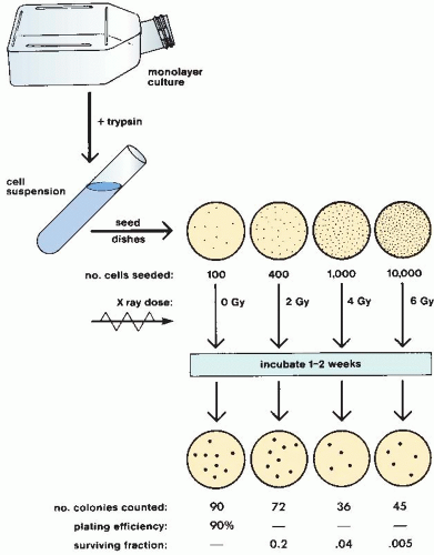FIGURE 3.2 The cell culture technique used to generate a cell survival curve. Cells from a stock culture are prepared into a single-cell suspension by trypsinization, and the cell concentration is counted. Known numbers of cells are inoculated into petri dishes and irradiated. They are then allowed to grow until the surviving cells produce macroscopic colonies that can be counted readily. The number of cells per dish initially inoculated varies with the dose so that the number of colonies surviving is in the range that can be counted conveniently. Surviving fraction is the ratio of colonies produced to cells plated, with a correction necessary for plating efficiency (i.e., for the fact that not all cells plated grow into colonies, even in the absence of radiation).

The extrapolation number, n, is a measure of the width of the shoulder. If n is large (e.g., 10 or 12), the survival curve has a broad shoulder. If n is small (e.g., 1.5-2), the shoulder of the curve is narrow. Another measure of shoulder width is the quasithreshold dose, shown as D_q in Figure 3.3. This sounds like a term invented by a committee, which in a sense it is. An easy way to remember its meaning is to think of the hunchback of Notre Dame. When the priest was handed the badly deformed infant who was to grow up to be the hunchback, he cradled him in his arms and said, “We will call him Quasimodo—he is almost a person!” Similarly, the quasithreshold dose is almost a threshold dose. It is defined as the dose at which the straight portion of the survival curve, extrapolated backward, cuts the dose axis drawn through a survival fraction of unity. A threshold dose is the dose below which
there is no effect. There is no dose below which radiation produces no effect, so there can be no true threshold dose; D_q, the quasithreshold dose, is the closest thing.

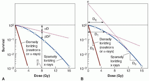FIGURE 3.3 Shape of survival curve for mammalian cells exposed to radiation. The fraction of cells surviving is plotted on a logarithmic scale against dose on a linear scale. For α-particles or low-energy neutrons (said to be densely ionizing), the dose-response curve is a straight line from the origin (i.e., survival is an exponential function of dose). The survival curve can be described by just one parameter, the slope. For x- or γ-rays (said to be sparsely ionizing), the doseresponse curve has an initial linear slope, followed by a shoulder; at higher doses, the curve tends to become straight again. A: The linear quadratic model. The experimental data are fitted to a linear-quadratic function. There are two components of cell killing: One is proportional to dose (αD); the other is proportional to the square of the dose (βD²). The dose at which the linear and quadratic components are equal is the ratio α/β. The linear-quadratic curve bends continuously but is a good fit to experimental data for the first few decades of survival. B: The multitarget model. The curve is described by the initial slope (D₁), the final slope (D₀), and a parameter that represents the width of the shoulder, either n or D_q.

At first sight, this might appear to be an awkward parameter, but in practice, it has certain merits that become apparent in subsequent discussion. The three parameters, n, D₀, and D_q, are related by the expression

The linear-quadratic model has taken over as the model of choice to describe survival curves. It is a direct development of the relation used to describe exchange-type chromosome aberrations that are clearly the result of an interaction between two separate breaks. This is discussed in some detail in Chapter 2.

The linear-quadratic model, illustrated in Figure 3.3A, assumes that there are two components to cell killing by radiation, one that is proportional to dose and one that is proportional to the square of the dose. The notion of a component of cell inactivation that varies with the square of the dose introduces the concept of dual radiation action. This idea goes back to the early work with chromosomes in which many chromosome aberrations are clearly the result of two separate breaks. (Examples discussed in Chapter 2 are dicentrics, rings, and anaphase bridges, all of which are likely to be lethal to the cell.)

By this model, the expression for the cell survival curve is

in which S is the fraction of cells surviving a dose D, and α and β are constants. The components of cell killing that are proportional to dose and to the square of the dose are equal if

This is an important point that bears repeating: The linear and quadratic contributions to cell killing are equal at a dose that is equal to the ratio of α to β.

A characteristic of the linear-quadratic formulation is that the resultant cell survival curve is continuously bending; there is no final straight portion. This does not coincide with what is observed experimentally if survival curves are determined down to seven or more decades of cell killing in which case the dose-response relationship closely approximates to a straight line in a log-linear plot; that is, cell killing is an exponential function of dose. In the first decade or so of cell killing and up to any doses used as daily fractions in clinical radiotherapy, however, the linear-quadratic model is an adequate representation of the data. It has the distinct advantage of having only two adjustable parameters, α and β.

▪ MECHANISMS OF CELL KILLING

DNA as the Target

Abundant evidence shows that the principal sensitive sites for radiation-induced cell lethality are located in the nucleus as opposed to the cytoplasm.

Early experiments with nonmammalian systems, such as frog eggs, amoebae, and algae, were designed so that either the cell nucleus or the cytoplasm could be irradiated selectively with a microbeam. The results indicated that the nucleus was much more radiosensitive than the cytoplasm.

Evidence for chromosomal DNA as the principal target for cell killing is circumstantial but overwhelming. There is evidence that the nuclear membrane may also be involved. Indeed, the one does not exclude the other because some portions of the DNA may be intimately involved with the membrane during some portions of the cell cycle.

The evidence implicating the chromosomes, specifically the DNA, as the primary target for radiation-induced lethality may be summarized as follows:

Cells are killed by radioactive tritiated thymidine incorporated into the DNA. The radiation dose results from short-range α-particles and is therefore very localized.
Certain structural analogues of thymidine, particularly the halogenated pyrimidines, are incorporated selectively into DNA in place of thymidine if substituted in cell culture growth medium. This substitution dramatically increases the radiosensitivity of the mammalian cells to a degree that increases as a function of the amount of the incorporation. Substituted deoxyuridines, which are not incorporated into DNA, have no such effect on cellular radiosensitivity.
Factors that modify cell lethality, such as variation in the type of radiation, oxygen concentration, and dose rate, also affect the production of chromosome damage in a fashion qualitatively and quantitatively similar. This is at least prima facie evidence to indicate that damage to the chromosomes is implicated in cell lethality.
Early work showed a relationship between virus size and radiosensitivity; later work showed a better correlation with nucleic acid volume. The radiosensitivity of a wide range of plants has been correlated with the mean interphase chromosome volume, which is defined as the ratio of nuclear volume to chromosome number. The larger the mean chromosome volume, the greater the radiosensitivity.

The Bystander Effect

Generations of students in radiation biology have been taught that heritable biologic effects require direct damage to DNA; however, experiments in the last decade have demonstrated the existence of a bystander effect, defined as the induction of biologic effects in cells that are not directly traversed by a charged particle, but are in proximity to cells that are. Interest in this effect was sparked by the 1992 report of Nagasawa and Little that following a low dose of α-particles, a larger proportion of cells showed biologic damage than was estimated to have been hit by an α-particle; specifically, 30% of the cells showed an increase in sister chromatid exchanges even though less than 1% were calculated to have undergone a nuclear traversal. The number of cells hit was arrived at by a calculation based on the fluence of α-particles and the cross-sectional area of the cell nucleus. The conclusion was thus of a statistical nature because it was not possible to know on an individual basis which cells were hit and which were not.

This observation has been extended by the use of sophisticated single-particle microbeams,
which make it possible to deliver a known number of particles through the nucleus of specific cells, whereas biologic effects can be studied in unirradiated close neighbors. Most microbeam studies have used α-particles because it is easier to focus them accurately, but a bystander effect has also been shown for protons and soft x-rays. Using single-particle microbeams, a bystander effect has been demonstrated for chromosomal aberrations, cell killing, mutation, oncogenic transformation, and alteration of gene expression. The effect is most pronounced when the bystander cells are in gap-junction communication with the irradiated cells. For example, up to 30% of bystander cells can be killed in this situation. The bystander effect is much smaller when cell monolayers are sparsely seeded so that cells are separated by several hundred micrometers. In this situation, 5% to 10% of bystander cells are killed, the effect being due, presumably, to cytotoxic molecules released into the medium. The existence of the bystander effect indicates that the target for radiation damage is larger than the nucleus and, indeed, larger than the cell itself. Its importance is primarily at low doses, where not all cells are “hit,” and it may have important implications in risk estimation.

In addition to the experiments described previously involving sophisticated single-particle microbeams, there is a body of data involving the transfer of medium from irradiated cells that results in a biologic effect (cell killing) when added to unirradiated cells. These studies, which also evoke the term bystander effect, suggest that irradiated cells secrete a molecule into the medium that is capable of killing cells when that medium is transferred onto unirradiated cells. Most bystander experiments involving medium transfer have used low-LET x- or γ-rays.

Apoptotic and Mitotic Death

Apoptosis was first described by Kerr and colleagues as a particular set of changes at the microscopic level associated with cell death. The word apoptosis is derived from the Greek word meaning “falling off,” as in petals from flowers or leaves from trees. Apoptosis, or programmed cell death, is common in embryonic development in which some tissues become obsolete. It is the mechanism, for example, by which tadpoles lose their tails.

This form of cell death is characterized by a stereotyped sequence of morphologic events. One of the earliest steps a cell takes if it is committed to die in a tissue is to cease communicating with its neighbors. This is evident as the dying cell rounds up and detaches from its neighbors. Condensation of the chromatin at the nuclear membrane and fragmentation of the nucleus are then evident. The cell shrinks because of cytoplasmic condensation, resulting from crosslinking of proteins and loss of water. Eventually, the cell separates into several membrane-bound fragments of differing sizes termed apoptotic bodies

Only gold members can continue reading. Log In or Register to continue