Clinical Cardiovascular Magnetic Resonance Imaging Techniques

The first dedicated cardiovascular magnetic resonance (CMR) clinical services opened in the United States in mid-1990s. Since that time, CMR imaging has become routine at most academic medical centers, with a number of centers now running multiple CMR scanners dedicated to cardiovascular imaging studies. Although different centers still differ somewhat with regard to the exact clinical CMR imaging protocols employed, in recent years cross-institutional CMR protocols have become much more consistent. In this chapter we focus on the clinical CMR imaging techniques that we routinely use at our institution, and we believe these are now representative of most high-volume dedicated CMR clinical services.

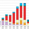
The dedicated CMR clinical service at the Duke Cardiovascular Magnetic Resonance Center (DCRMC) first opened in July 2002. Since that time, we have experimented with and evaluated many approaches to CMR and have directly observed their effects on overall clinical volume. As shown in Fig. 14.1 , clinical volume at the DCRMC has grown steadily since our service first opened and currently consists of approximately 4000 billed CMR imaging procedures per year.

From 2002 to 2010 the percentage of each type of CMR test we performed varied somewhat as the types of patients referred to us evolved, and as we ourselves modified the tests we offered. From 2010 to 2015 (the latest year data are available), however, the tests we offer and perform have remained relatively constant.

Fig. 14.2 summarizes the indications for CMR scans, as well as the corresponding current procedural terminology (CPT) codes used for billing. These data were pooled across four US hospitals with dedicated CMR clinical services and, as such, portray an arguably representative picture of clinical practice patterns in the United States. The largest referral indication for CMR was heart failure, followed by ischemia evaluation and vascular disease. The most common CPT codes were 75561 (morphology and function with/without contrast), 75565 (velocity flow), and 71555 (magnetic resonance angiography [MRA]). About 20% of all CMR scans involved stress testing (CPT code 75563). Unlike the four-hospital data of Fig. 14.2 , however, at our institution roughly 50% of our CMR scans involve stress testing. The DCMRC definition of a “CMR Stress Test” can briefly be described as a group of three individual scans:

1.

Cines (to examine biventricular contractile function).
2.

Adenosine stress/rest perfusion (to examine regional myocardial perfusion).
3.

Late gadolinium enhancement (LGE; to examine viability/infarction).

The DCMRC CMR Stress Test is described in more detail in a paper by Klem et al., and has arguably become the bread and butter of our clinical service.

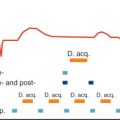
Through the years our philosophy about how to perform CMR has evolved into the concept of a CMR “exam menu” which has not only allowed us to streamline our clinical service but has also made it considerably easier for us to teach CMR to cardiology fellows and level 2 trainees. The underlying idea of the examination menu ( Fig. 14.3 ) is that most if not all routine clinical CMR can be performed simply by combining one or more items from a predetermined menu and performing these scan protocols/pulse sequences in a single consistent manner. As can be seen from Fig. 14.3 , the CMR Stress Test is simply one combination of items from the examination menu. Virtually every patient we examine simply undergoes one or more of the items shown in the menu and, perhaps more importantly, only rarely do we find it necessary to perform a scan not listed there.

Accordingly, the remainder of this chapter focuses on providing more detail about each of the items on the examination menu, with an emphasis on providing practical information typically not provided in other CMR textbooks. In the Conclusion section of this chapter we present typical examples of how the items on the examination menu can be combined to answer common diagnostic questions in cardiology, such as the detection of coronary artery disease (CAD) and the evaluation of aortic disease.

Scouting (“Scan” = “Scout”)

The thoracic scout examination is the simplest and most commonly used CMR procedure performed during the CMR examination. The goal of the scout examination is to establish the anatomic position of the heart and the short-axis and long-axis views of the heart. Anatomic variations from patient to patient cause both the short-axis and long-axis cardiac views to lie at arbitrary angles with respect to scanner coordinates. These views are then obtained using “double oblique” planes.

The first step in determining the proper double-oblique views is to acquire images along the axes of the scanner: that is, axial, sagittal, and coronal planes passing through the thoracic cavity. Fig. 14.4 shows typical examples of scout images. These scout images are used to prescribe single-oblique images: that is, perpendicular to the axial image of Fig. 14.4 , going through the left ventricle (LV) parallel to the septum (dashed yellow line). The single-oblique images (pseudo two-chamber and pseudo four-chamber views) are used to determine the true short axis of the heart (doubly oblique). Therefore the goal of the scout is to acquire a series of images similar to that of Fig. 14.4 which define the short and long axis of the heart.

The pulse sequence we use for the scout images is based on balanced steady-state free precession (bSSFP). The underlying concept of bSSFP was described in the mid-1980s but only since the late 1990s has CMR scanner hardware been capable of achieving the bSSFP magnetization state. Fig. 14.5 shows the bSSFP pulse sequence timing diagram characterized by its elegant simplicity, with symmetry around the data acquisition window on all three gradient axes. The axis labeled “slice” serves to select the slice to be imaged. The waveforms on the “read” axis create the magnetic resonance (MR) signal as an echo (see “signal” axis on bottom). During the positive portion of the “read” waveform the MR signal is digitally sampled. The “phase” encoding axis imposes a different phase on each echo which allows spatial encoding of the second dimension called y in Fig. 14.6 . In practice, the primary advantages of bSSFP imaging are: (1) fast imaging (i.e., short repetition time [TR]) and (2) very high signal-to-noise ratio (SNR) images. Accordingly, we use bSSFP not only for scouting but also for cine imaging (described in the Contractile Function section).

Acquiring any CMR image in essence involves filling the raw data space, often referred to as “ k -space.” Fig. 14.6 graphically depicts the process of filling k -space as a series of “lines” starting at the top and proceeding to the bottom. Each line is actually one echo (see zoomed-up box) acquired during the read event (“read” signal in Fig. 14.5 ). The echo runs in the x -direction. The y -dimension is the phase-encoding direction. For a bSSFP pulse sequence running on a typical modern CMR scanner the time needed to acquire each k -space line is approximately 3 ms. So, for the 100 k -space lines typical for scouting, the total image acquisition time is ~300 ms (100 × 3) or one-third of a second. This is fast enough to effectively freeze heart motion provided that the image data are acquired during diastole when the heart is relatively quiescent.

Acquiring the image data in diastole requires that the scanner hardware is “gated” to the cardiac cycle. This is typically achieved by having the scanner detect the R-wave of the electrocardiographic (ECG) signal and initiating the scan sequence at that time. In the following scouting example we assume a heart rate of 60 beats per minute (RR duration = 1000 ms). The first “event” the scanner hardware must play out is a delay time of approximately 500 ms after the QRS (to get to diastole), followed by the 300 ms of image data acquisition. Fig. 14.7 graphically depicts cardiac gating for scout imaging.

Morphology (“Scan” = “Morphology”)

CMR scanning for cardiac morphology is used less often than cine imaging or even viability imaging, but the technical aspects of morphology, particularly as it relates to cardiac gating, are only modestly more complex than for scouting, so we present these next.

The “goal” of morphology scanning is essentially to create a series of parallel slices which “bread loaf” the thoracic cavity to examine vascular anatomy. Typically, three sets of black-blood and bright-blood images are acquired in the axial, coronal, and sagittal orientations. Once acquired, the scanner operator can then step through each series of image slices and understand the patient’s vascular anatomy as well as plan additional scan planes.

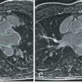
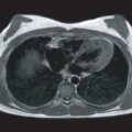
It is often desirable to do this both with “black-blood” imaging ( Fig. 14.8 ) and with “bright-blood” imaging ( Fig. 14.9 ). The CMR pulse sequences used for black-blood and bright-blood morphology imaging are half-Fourier acquisition single-shot turbo spin echo (HASTE, Fig. 14.10A ) and bSSFP ( Fig. 14.5 ), respectively. Fig. 14.10A shows the pulse sequence timing diagram of the turbo spin echo sequence, and Fig. 14.10B shows the simplified spin echo sequence. HASTE is a special variant of the turbo spin echo sequence in which only 60% of k -space is sampled to reduce acquisition time.

Cardiac ECG gating for bSSFP morphology images is the same as that used for scouting, namely, by acquiring the entire image during a single diastolic phase ( Fig. 14.11 ). For example, a set of 40 bSSFP images for morphology would require 40 consecutive heartbeats. ECG gating for HASTE imaging is also performed in diastole; however, these images are typically acquired every other heartbeat (e.g., 80 consecutive heartbeats). HASTE images require additional heartbeats to satisfy the black-blood imaging condition (described later). Morphology imaging typically takes 3 to 5 minutes and is performed with quiet respiration. For example, the acquisition of the 40 slices with both bSSFP and HASTE slices would take 40 + 80 = 120 heartbeats (i.e., about 2 minutes).

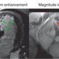
Black-blood imaging is often advantageous for the examination of morphology because it allows clear differentiation of the inner portion of the vessel wall from the blood. Black-blood HASTE can be achieved by carefully combining CMR physics with the physiology of moving blood. The underlying reason that the blood appears black in HASTE images is caused by preparatory radiofrequency (RF) pulses before the HASTE readout (see Fig. 14.10 ). The basic concept is graphically depicted in Figs. 14.12 and 14.13 . Soon after the R-wave, a brief (1–3 ms) RF pulse is played, which causes all of the magnetization in the body (“nonselective” or “hard” pulse) to flip upside down (“180 degrees” or “inversion” pulse). Immediately after this, a second RF pulse is played, which causes only the magnetization within the prescribed imaging slice to flip back to where it started (“slice-selective” re-inversion pulse). The net effect of these preparation pulses results in the magnetization outside the slice being inverted, whereas the magnetization within the prescribed imaging slice is restored. During the interval between the preparatory pulses and the HASTE readout (see Fig. 14.13 ) the heart contracts and expels blood from the slice (see Fig. 14.12 , middle ), which is subsequently replaced by fresh blood from outside the slice (see Fig. 14.12 , right ), which was previously inverted. When the HASTE readout begins, the previously inverted blood is recovering with T1, and its curve crosses zero at the start of the HASTE readout. Consequently, the blood produces no signal and appears black. Thus black-blood HASTE is made possible by a clever combination of a “memory” effect related to CMR physics (T1 recovery) as well as to the physiology of moving blood (and therefore may have intermediate signal with stagnant blood flow). Such images are quite helpful in detecting abnormalities in large-vessel anatomy, especially when combined with bright-blood bSSFP images at the same location.

Contractile Function (“Scan” = “Cine”)

Contractile function is a fundamental part of the CMR examination. Contractile function imaging is used for global and regional wall motion assessment and has been demonstrated to be highly accurate and reproducible for LV and right ventricular (RV) volume, ejection fraction, and mass measurements. In recent years, CMR has become widely accepted as the clinical gold standard for contractile function assessment. It has been used as an endpoint for the evaluation of ventricular remodeling, and as a reference method for other imaging techniques.

The “goal” of cine imaging is to capture a movie of the beating heart to visualize its contractile function. Fig. 14.14 shows a representative example of a mid-ventricular short-axis slice during different time points within the cardiac cycle, from early systole to late diastole. Images are acquired with the same bSSFP sequence used in bright-blood and scout imaging (see Fig. 14.5 ). The advantage of bSSFP for cardiac function imaging is high SNR, high temporal resolution, and excellent blood–myocardium contrast, which helps identify the endocardial border. Typically, a stack of multiple short axis slices (5–6 mm thick) are acquired at 1-cm increments to provide full LV and RV coverage. Short-axis views can be planned perpendicular to the long-axis scout images described in the Scouting section. In addition, cine images can be obtained in multiple long-axis views such as the two-chamber, three-chamber, and four-chamber views.