Component Analysis for the Classification of Cardiac Motion Abnormalities Based on Echocardiographic Strain and Strain Rate Imaging

) with a GE VingMed Vivid7 equipped with a 2.5 MHz transducer. For each subject, data were acquired in the apical 2-, 3- and 4-chamber views with optimization of the pulse repetition frequency in order to avoid aliasing. An event-driven graphical user interface called SPEQLE [4] was used for the post-processing of the data to extract longitudinal strain (rate) traces in an 18-segment model of the left ventricle [2]. Since the number of samples of the extracted curves could be different due to the differences in the heart rates of the subjects, a linear interpolation procedure was adopted to have the same number of samples in all traces. To avoid unwanted changes of the curves due to the interpolation procedure, each of the six cardiac phases (i.e. electromechanical coupling, isovolumetric contraction, ejection, isovolumetric relaxation, early filling and late filling [6]) was interpolated separately and then merged to have the whole heart cycle. The interpolated curves were then used in the PCA implementation and classification phases.

Table 1 lists the number of subjects that were selected randomly from the healthy and pathological groups for building training, validation and test sets. This random selection was repeated 10 times and the results presented in Sect. 3 are the average of running the classifier on these 10 different sets of data. Since for a pathological subject only the subset of acutely infarcted segments was used for the classification task, the number of utilized pathological subjects in Table 1 was more than the healthy ones so that both groups had roughly the same number of curves in the training, validation and test sets. Note that, the segmental strain and strain rate curves were sorted in two different groups of training, validation and test data to study their clinical relevance for discriminating normal and infarcted traces.

Table 1.

Number of subjects taken from the healthy and pathological groups for the training, validation and test sets

	$\#$ Training	$\#$ Validation	$\#$ Test
Healthy subjects	12	5	10
Pathological subjects	25	9	20

2.2 Principal Component Analysis

PCA is a popular statistical approach for feature extraction, dimensionality reduction and data visualization [8, 12]. Given a data set of random vectors $X = \lbrace x_1 \dots x_N \rbrace$ where $x_i \in \mathbb {R}^ n$ , the PCA algorithm gives a representation of the data in $\mathbb {R}^ m$ (

) such that the new variables are less redundant compared to the original ones.

The first step in building the PCA model is centering the data that can be done by first computing the mean vector of X and then subtracting every data vector from it. In the second step, the covariance matrix of the centralized data set is computed. The third step is to find the $n \times n$ eigenvector matrix $\varPhi = \lbrace \phi _1 \dots \phi _n \rbrace$ and diagonal eigenvalue matrix $\varLambda = diag \lbrace \lambda _1 \dots \lambda _n \rbrace$ of the covariance matrix. The final step is to insert the first m eigenvectors of $\varPhi$ with the largest eigenvalues, which are known as Principal Components (PCs), into a new matrix $\varPsi$ and project the data onto the space spanned by the eigenvectors of $\varPsi$ ,

$\begin{aligned} Y = \varPsi ^T \overline{X} \end{aligned}$

(1)

where the variance of the new low-dimensional data Y is maximized which means that the first axis has the largest variance, the second axis has the second largest variance and so on.

2.3 Classifier

Performance of a classification system depends on both the features extracted from the data and the classification technique. In order to differentiate between the effects of the employed features and the classification strategy on the final classification outcomes, two different classifiers are used in our experiments. The first classifier is called the locan-mean based (LMB) method [11] and considers the information of classes around a test sample for its classification. The second classifier is support vector machine (SVM) [5]. It works based on the idea of the maximum margin solution and finds a hyper-plane that has the greatest distance to the training samples in the boundaries of a binary classification problem.

3 Results

3.1 PCA Outcomes

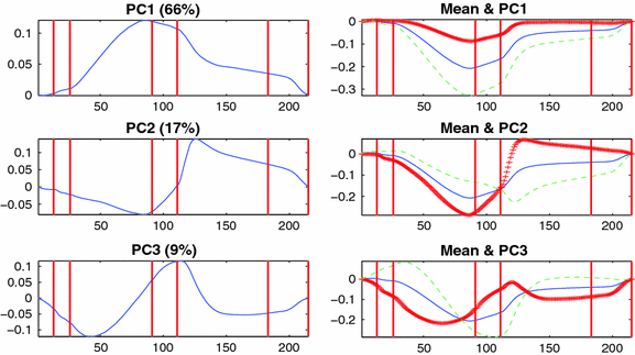
The segmental strain and strain rate traces of the training sets were used to build two separate PCA models. Figures 1 and 2 illustrate the first three PCs of the strain and strain rate traces, respectively. The variance percentages accounted for the PCs and the results of adding and subtracting the PCs to and from the mean curves are also showed. In order to investigate the PCs’ structures in terms of timing of the six mechanical phases of the cardiac cycle, the timing of the onset of each phase is shown with a red vertical line.