Computed Tomography

Computed tomography (CT) has experienced enormous growth in clinical use over the past three decades (Fig. 10-1) primarily due to significant advances in image quality and a dramatic (1,000 fold) reduction in acquisition time as the technology has advanced. Image quality has increased as a result of better detector sampling along the long axis (z-dimension) of the patient when multiple detector array systems were developed. CT reconstruction has also advanced from filtered backprojection (FBP) to different generations of iterative reconstruction, and now deep learning (DL)-based adjuncts to the CT reconstruction process have led to lower noise images at lower radiation dose levels. Many other subtle technologies, discussed in this chapter, have also led to better spatial resolution and contrast resolution in CT. CT acquisition times have plummeted with the advent of helical scanning (continuous table movement), combined with multiple detector array CT systems that allow 40 mm (or greater) sections of the patient to be imaged in one rotation of the gantry. With half-second gantry rotation (or shorter), 80 mm of patient length can be acquired in 1 second (s), and hence 400 mm of patient length can be scanned in 5 s. The speed of the CT examination is one of the factors that has driven its clinical use as shown in Figure 10-1.

These technical advances have allowed CT imaging to gain widespread use across many clinical applications, and the medley of CT images illustrated in Figure 10-2 shows the broad application of CT technology to abdominal, thoracic, head, musculoskeletal, and many other imaging applications. High temporal resolution CT can allow CT angiography (CTA) or organ specific CT perfusion. Dual energy CT allows 3D reconstruction and segmentation of bone structures from soft tissue, with accurate assessment of iodinated contrast agent concentration over time in three dimensions. Dual energy CT also allows physicians to characterize gout, and is used in radiation therapy treatment planning for assessment of electron density.

Conventional CT scanners scan along the z-dimension (long axis) of the patient’s body or head with a gantry rotating rapidly around the patient. This acquisition geometry leads to a reconstruction plane in the axial plane of the patient. A single abdominal CT image is shown in Figure 10-3, and the axial plane corresponds to the principal reconstruction plane of most CT scanners—coronal and sagittal CT images are typically synthesized from the reconstructed (thin section) axial CT images. The two-dimensional image shown is comprised of individual pixel elements (pixels), and typically each pixel has equal dimensions in the horizontal (x) and the vertical (y) dimensions. The two-dimensional CT image corresponds to a volumetric section of the patient’s body, which has a given thickness (Δz) depending upon acquisition and reconstruction parameters. Hence, each pixel in the image corresponds to a volume element or voxel in the patient’s body. For normal resolution (NR) CT scanner, the dimensions of each voxel can be on the order of 0.60 mm (Δx and Δy) by 0.50 mm (Δz)—corresponding to 0.18 mg of unit-density tissue. Hence, a 75-kg person can be imaged using over 400 million voxels using CT.

Because of the small in-plane pixel dimensions (Δx, Δy) and the correspondingly small slice thickness (Δz), the volume data set of axial CT images are routinely
reformatted from the original (axial) reconstruction plane into both coronal and sagittal images (Fig. 10-4), allowing the radiologist to view truly orthogonal images, which provide a more intuitive impression of patient anatomy. The ability to routinely visualize both coronal and sagittal CT images provides important additional information to the interpreting physician, including spinal alignment, orientation of pathology and normal anatomy including identifying feeding vessels, gastrointestinal tract topography, abdominal organ placement and orientation, trauma, and other factors.

▪ FIGURE 10-1 The number of CTs performed annually in the United States is illustrated for almost 3 decades. The dramatic increase in the use of CT demonstrates both the clinical utility of the modality, as well as increases in technical performance, such as better image quality and shorter acquisition times. The fluctuation in the curve from 2012 onward is the result of some concerns over radiation dose, but primarily is due to changes in reimbursement related to exam bundling (and hence how CT examinations are counted).

10.1 BASIC CONCEPTS

X-ray CT scanners typically run at 120 kV for routine scanning; however, the x-ray tube voltage can be varied to optimize the trade-off between image quality and radiation dose for different clinical imaging applications and different patient sizes. This
allows the development of protocols that are very patient-specific. The high kV combined with the added filtration in the x-ray tube leads to a relatively “hard” x-ray spectrum—one with relatively high effective energy. The tube voltage options in CT depend on the vendor; however, 80-, 100-, 120-, and 140-kV spectra are typical (but not exclusive) in the industry (Fig. 10-5). The high x-ray energy used in CT is important for understanding what physical properties of tissue are being displayed on CT images. The effective energies of the four spectra illustrated in Figure 10-5 range from about 43 to 70 keV, and this region is overlaid on the mass attenuation coefficients for soft tissue in Figure 10-6. In this region, it is seen that Rayleigh scattering and photoelectric effect have the lowest interaction probability and the Compton scatter interaction has the highest interaction probability. Also visible from the figure, it is seen that the Compton scattering interaction is 10-fold more likely than the photoelectric effect in soft tissue (the atomic number dependent photoelectric effect does

play a larger role in x-ray photon attenuation in bone, metal implants, and iodinated contrast agent). For soft tissue, the CT image grayscale (also known as CT number or Hounsfield Unit) represents the physical property for which Compton scattering is most dependent on, which is electron density. As discussed in Chapter 3, the Compton scatter linear attenuation coefficient, µ_Compton, is proportional to

where ρ is the mass density of the tissue in a voxel, N is Avogadro’s number (6.023 × 10²³), Z is the atomic number, and A is the atomic mass. The primary constituents of soft tissue are carbon, hydrogen, oxygen, and nitrogen, and the Z/A ratio for most of these elements is ½. For hydrogen, however, the Z/A ratio is 1. While this would imply that hydrogenous tissues such as adipose tissue would have a higher µ_Compton, in reality, hydrogen content in tissues is small and the lower density of adipose (ρ ≈ 0.94 g/cm³) relative to soft tissue (ρ ≈ 1) tends to dominate Equation 10-1 when it comes to the difference between soft tissue and hydrogen-rich adipose tissues. Consequently, adipose tissue appears darker (has a lower µ_Compton) than soft tissues such as liver or other organ parenchyma (see Fig. 10-4).

▪ FIGURE 10-2 The high spatial resolution and excellent contrast resolution of modern CT systems, as illustrated on this medley of images, have contributed to the clinical demand for CT imaging. While the primary forte of CT imaging is fundamental three-dimensional anatomical imaging, with the addition of iodinated contrast, functional imaging including enhancement and perfusion metrics can be assessed quickly, accurately, and quantitatively.

▪ FIGURE 10-3 Individual CT images (with axial images shown here) are comprised of a two-dimensional matrix of picture elements, referred to as pixels. For most CT images, Δx and Δy are identical due to the nature of the reconstruction. While the individual CT image is typically a two-dimensional presentation, each pixel in the image corresponds to a volume element or voxel in the patient. The Δz dimension of a voxel typically is slightly different from the Δx or Δy dimension, because of differences in the geometry of CT acquisition.

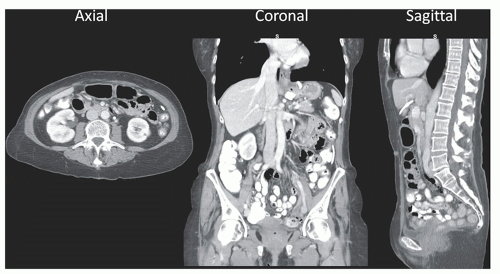▪ FIGURE 10-4 In the earlier days of CT technology, the slice thickness of the images (Δz in Fig. 10-3) was typically much larger than the in-plane (Δx or Δy) voxel dimensions, and this limited the majority of image interpretation to the axial image presentation. With modern CT systems, dimensions of Δz can be smaller than the in-plane voxel dimensions, and consequently the presentation of both coronal and sagittal images (along with axial images) is typical in modern viewing environments.

▪ FIGURE 10-5 The x-ray spectra for computed tomography are shown for 80, 100, 120, and 140 kV—each spectrum is filtered with 10 mm of aluminum, which approximates the typical amount of filtration at the center of the beam for most CT scanner models. The high tube potentials along with the large filtration thicknesses lead to x-ray beams with high effective energy.

▪ FIGURE 10-6 What physical parameter does the grayscale in a CT image correspond to? The mass attenuation coefficient of soft tissue is shown as a function of x-ray energy in this graph. The curves correspond to the attenuation coefficients for the photoelectric effect, Rayleigh and Compton scattering. The effective energy in CT is outlined by the vertical band. In this region, it is seen that the Compton cross section is approximately tenfold that of the Rayleigh or photoelectric cross sections, meaning that the gray scale (Hounsfield Unit) in CT for soft tissue is primarily determined by the physical dependency of Compton scattering—electron density.

While radiographic modalities tend to demonstrate the exponential attenuation properties of tissues, the preprocessing steps and subsequent reconstruction used in CT lead to grayscale in CT, which is a linear function of the linear attenuation coefficient. Indeed, the grayscale in CT is given a special name Hounsfield Unit (or HU) after one of the principal developers of the technology, Sir Godfrey Hounsfield. The Hounsfield Unit is scaled as described in Equation 10-2:

For a given voxel K in the image, which contains tissue with an average linear attenuation coefficient µ_K, the Hounsfield Unit is scaled relative to the linear attenuation coefficient of water, µ_w. The linear attenuation coefficient of water, µ_air, is also used in the definition; however this value is so small that it is negligible (as the rightmost term in Eq. 10-2 shows). The scaling shown in Equation 10-2 defines the HU range at two physically meaning points: it can be seen that if voxel K contained only pure water, then µ_K = µ_w, and thence HU_K = 0. If voxel K contained only air, then µ_K ≈ 0, and HU_K = -1,000.

The linear attenuation coefficient has relatively strong dependencies on the x-ray beam energy (Fig. 10-6), and so could be written as µ_w(E). Equation 10-2 avoids this notation by inferring that the linear attenuation coefficients in the equation represent the effective linear attenuation coefficient, µ_eff. With this in mind, it should be noted that the calibration of the Hounsfield Unit is different for each x-ray tube potential used in CT, and thus the value of µ_w-eff changes (slightly) for 80 kV, 100 kV, etc. While for water, HU = 0, always; other tissues such as liver and bone will have slightly different HU values at different tube potentials.

The ideal for each CT scanner is that HU_w = 0; however the impact of many other factors (calibration, scattered radiation, quantum noise, beam hardening, etc.) mean that water will in fact have a range of HU values, for example HU_w ≈ ±5. It is also true in principle that for air, HU_air = -1,000; however air is relatively unique in CT. For example, the bowel will often contain large pockets of air, but during CT acquisition x-ray scatter from surrounding tissues will be detected in the same detector elements where the shadow of air should be recorded. This leads to an increase in HU_air, which can often be in the -800 to -900 range for air voxels in the bowel.

In the early days of single detector array CT, the x-ray beam was typically collimated to 5 mm at the isocenter of the scanner, and this narrow-beam geometry allowed for excellent scatter rejection. Today, in the era of multiple detector array CT, the collimated x-ray beam can be 40 mm wide, or even greater. This means that modern CT scanners don’t have the same scanner rejection properties as the earlier scanners, and scattered radiation that is recorded by the detectors can lead to substantial imprecision in HU values.

10.2 CT SYSTEM DESIGNS

10.2.1 The Gantry—Geometry and Detector Configuration

Most clinical CT scanners have detector arrays that are arranged in an arc across from the x-ray tube, as shown in Figure 10-7. This arc is efficient from several standpoints—firstly, by mounting the detector modules on a support structure that is aligned along a radius of curvature emanating from the x-ray source, there is very little difference in fluence to the detectors due to the inverse square law. Very importantly, the primary x-rays strike the detector elements in a nearly normal manner, and so there is effectively no x-ray beam parallax that can reduce spatial resolution. Figure 10-7 also defines a fan beam projection. The individual rays in this geometry each define a line integral that extends between the x-ray source and each individual x-ray detector along the detector array. A collection of these rays across all the detector elements constitutes a view (or projection) that is specific to the view angle at which the data are acquired and which changes as the gantry rotates around the patient. Rays and views make up the fundamental raw data collected during CT acquisition.

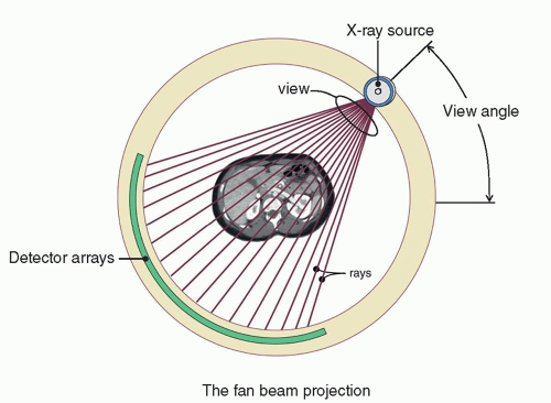▪ FIGURE 10-7 The general configuration of a CT scanner is illustrated in cross section. The x-ray tube is mounted on a rotating gantry, onto which the x-ray detector arrays are also mounted, in the typical rotaterotate (third generation) geometry of all modern CT scanners. The x-ray tube and detector arrays rotate together in a fixed geometrical orientation. The x-ray source fan projects a beam of x-rays, which, after transmission through the patient, reach the detector and record the raw acquired signal. The line between the x-ray source and each individual detector element (dexel) corresponds to the fundamental measurement in CT, a ray. The group of rays corresponding to one fan-beam projection is called a view. Rays and views are the fundamental data in CT imaging.

▪ FIGURE 10-8 Some of the basic geometrical dimensions of a modern rotate-rotate CT scanner are shown. The detector arrays are located on a radius-of-curvature positioned a distance B from the x-ray source. The source-to-isocenter distance is given by a distance A, and hence the magnification factor (M) of objects at isocenter are given by the ratio M = B/A. For most modern CT scanners, the fan angle is about 50°-60°, and combined with the other geometric parameters this defines the maximum field-of-view (FOV).

Figure 10-8 illustrates some basic geometry pertinent to CT scanners. The isocenter is the center of rotation of the CT gantry, and in most cases (but not all), the isocenter is also the center of the reconstructed CT image—that is, pixel (256, 256) on the 512 × 512 reconstructed CT image. The source-to-isocenter distance is illustrated as A in Figure 10-8, and the source-to-detector distance is labeled B. The magnification factor M from the isocenter to the detectors is then given by M = B/A. By convention in the industry, detector width and length and the collimated beam width are quoted at the isocenter. For example, if the (minimum) nominal CT detector thickness is quoted on a scanner as 0.50 mm, the physical detector width is larger by the magnification factor M. Thus, for this 0.50-mm nominal detector with B ≈ 95 cm and A ≈ 50 cm, then the M = 1.9 and the physical width of the detector array is M × 0.50 mm = 0.95 mm. Most whole body CT systems make use of the gantry system with a fan angle on the order of 50°-60°. The fan angle, combined with the source-to-isocenter and source-to-detector distances, defines the maximum field of view (FOV) obtainable by the CT system. Some CT systems are designed to have larger fields of view, for example for bariatric imaging or treatment planning in radiation therapy, where it is typical to have the patient’s arms positioned along their side which creates the need for a larger FOV. In diagnostic imaging of the torso, if they are able to, the patients typically raise their arms above their head, which reduces artifacts and reduces the FOV requirements.

Figure 10-9 illustrates gantry components on a modern multidetector array CT scanner (MDCT). A single detector array CT scanner has only one detector array which spans the fan angle—and that technology was the dominant configuration from the 1970s until the mid-1990s. Most modern CT systems use MDCT geometry, where 16, 64, 128, or more detector arrays are aligned next to each other along the fan angle. Because multiple detector arrays are abutted next to each other on the gantry, extending the total width of the detector assembly, a divergent x-ray beam in the z-axis giving rise to the cone angle (Fig. 10-9) results. For a 64 detector array CT scanner with 0.625 mm individual detector width, the thickness (along z) of the entire detector array measures 40 mm (defined at isocenter), since 64 × 0.625 mm = 40 mm. A newly introduced high-resolution CT scanner uses 160 detector arrays that are 0.25 mm in width, also spanning 40 mm (160 × 0.25 mm = 40 mm).

While a given CT scanner may have n detector arrays (e.g., n can be 64), most systems allow a configuration that “bins” the signals from adjacent detector arrays to produce lower z-axis resolution CT images (e.g., n/2). Using the high-resolution CT system mentioned above as an example, the system has acquisition modes including 160 × 0.25 mm and 80 × 0.5 mm, with progressively reduced resolution in z as the effective detector width increases. One may ask why any imaging system would
intentionally acquire data in a lower resolution mode. In CT, the finer detector spacing leads to larger data sets, which increases reconstruction time and can increase the number of CT images produced for a given FOV, which increases requirements on bandwidth for transfer as well as computer storage issues. Also, there are many clinical protocols where high resolution simply is not required for the diagnostic task at hand. But one of the most important reasons why some CT scanners allow detector binning modes is that the electronic noise can be reduced. This is because, using the high resolution CT scanner (HRCT) example above, when the signal from two adjacent 0.25 mm detector arrays is added to form an effective detector array width of 0.50 mm, electronic noise is reduced (relative to the signal) prior to the gain stages in the electronics that ultimately lead to the final digitization of the signal. This effect is over and above the issue of x-ray quantum noise versus slice thickness, which will be discussed later.

▪ FIGURE 10-9 This figure defines the angles associated with a modern rotate-rotate CT scanner using multidetector arrays. The fan angle is defined between the x-ray source and the extent of the detector arrays in-plane. All modern multiple detector array CT scanners (MDCT) can be considered cone beam CT systems, with full cone angles of 4.2° for a 40-mm detector width at isocenter, and 17.2° for a 160-mm detector width. This cone angle is fully considered in the reconstruction algorithm used to convert the raw acquired data into the final CT volume data set.

With MDCT, the reconstructed slice thickness and collimated x-ray beam width are separate parameters—acknowledging some practical clinical constraints, they are largely decoupled. This was not the case in the era of a single detector array CT, where the slice thickness in the reconstructed images was essentially equal to the collimated beam width. A thinner slice thickness improves resolution but required long scan times in these scanners, while wider beam widths make for faster scanning but offered decreased resolution. Thus, a significant compromise was necessary in the single detector array CT era between scan time and z-axis spatial resolution. By almost completely decoupling these parameters with MDCT, the slice thickness is primarily determined by the detector array configuration, and the x-ray beam width is determined by the collimator (along with the total width of the detector arrays). This leads to thinner slices and faster scans, a noteworthy combination made possible by multiple detector array CT. Examples will be given to illustrate this.

Faster Scans

In the standard terminology of CT, the detector thickness is T (measured at isocenter) and the number of detector arrays is n. For one manufacturer’s 64 slice (n) scanner, T = 0.625 mm and so the collimated x-ray beam width is nT = 40 mm. For contiguous images, the scan for a 320-mm length (along z) of a patient’s abdomen could be acquired in just 4 s (e.g., 40 mm beam width, ½ s gantry rotation, helical pitch = 1.0), since 80 mm of patient length along z can be scanned in 1 s. In practice, the scan would take perhaps 4.5 s due to over-ranging, which will be described later.

Thinner CT Images (Improved z-Axis Resolution)

For an NR scanner, the 40-mm beam width discussed in the above section can produce 0.625 mm thick images. For the 320-mm section of the abdomen discussed above, this would lead to 512 images. It should be noted that it is not always desirable to reconstruct the thinnest slice possible, due to the increase in quantum noise that is associated with thinner slices. More about this will be discussed later.

10.2.2 Wide Beam (Cone Beam) CT Systems

All top of the line (≥64 detector channels) whole body CT systems are technically cone beam CT systems, as the reconstruction algorithm used for synthesizing the raw data into CT images takes into account the cone angle. However, most conventional (˜64 slice) CT systems still make use of only slight cone angles on the order of ˜2° (cone beam half-angle). Some vendors, however, have developed what could be called true cone beam CT scanners—where the half cone angle approaches 9°. For example, some vendors have developed multiple-detector array systems with z-axis coverage (nT) of 16 cm. There are of course benefits and trade-offs with such wide cone beam designs. The challenges of wide cone beam imaging include increased x-ray scatter and increased cone beam artifacts. The benefit of this design, however, is that whole organ imaging can be achieved without table motion—so for CTA or CT perfusion studies, the anatomical coverage is sufficient for most organs (e.g., head, kidneys, heart, etc.) to be imaged in a single rotation. Hence, with these systems whole-organ perfusion imaging with high temporal resolution is possible.

Some niche CT scanners make use of flat panel detectors for the detector array, and an example of this (for breast CT) is shown in Figure 10-10. This geometry represents a full cone beam geometry, where the cone angle is almost as large as the fan angle. The use of the planar flat panel detector system leads to a fully two-dimensional bank of detectors, which have no curvature, and so a slightly different reconstruction geometry is required. This means that techniques (such as flat-fielding) are needed to correct for the inverse square law and heel effect-based spatial differences in fluence to the detector. There is also some parallax (non-normal x-ray incidence onto the detector) that occurs in this geometry, which cannot be corrected for.

Flat panel detectors have on the order of 3 million pixels, and hence the read out rate is much slower than purpose-built CT detector arrays. Because of this, most cone beam CT systems use a pulsed x-ray tube output to improve spatial resolution. In contrast, most whole body CT systems use continuously-on (non-pulsed) x-ray tube control.

The cone angle that exists with some flat panel based cone beam scanners can be appreciable; for example, using a standard 30 × 40 cm flat panel detector at a source-to-detector distance of 90 cm, the full fan angle spans about 25° and the full cone angle spans about 19°. Flat panel detectors are used for cone beam systems in dental and maxillofacial CT, breast CT, orthopaedic, angiographic, and radiation therapy imaging applications.

▪ FIGURE 10-10 While modern whole-body CT systems are rightly considered as (small cone angle) cone beam systems, more traditional specialty application cone beam CT systems typically use a flat panel detector opposed to an x-ray source in a rotate-rotate (third generation) cone beam geometry, as illustrated. The system in this diagram is designed for pendant-geometry breast imaging and rotates in the horizontal plane. Flat panel based cone beam CT systems enable dedicated CT applications in orthopedic, dental, breast, radiation therapy positioning, and angiographic applications, and typically provide higher spatial resolution images albeit with greater artifact potential.

10.2.3 The Slip Ring

Figure 10-11 shows a diagram of a modern slipring used in virtually all state-of-the-art CT scanners. The slipring itself interfaces with the rotating gantry, and it has a number of large brass tracks that carry electrical current at high voltage from a gliding contactor. The contactor is similar to the brushes that are used in an automobile generator. The large tracks on the slipring are used to maintain electrical contact with, and conduct electrical power from, the stationary frame to the rotating gantry. There are also numerous small tracks of the slipring that are used to conduct low-power (digital) signal data off of the rotating gantry to the stationary frame.

The use of the slipring in CT scanner design enables the gantry to rotate continuously in one direction. Prior to the use of sliprings, the rotating frame of the CT system was connected to the stationary frame using cables that extended and retracted on cable spools. Both thick power cables and thin ribbon cables for signal conduction were used. This mechanical linkage allowed about 720° of rotation. With these cables, the gantry was accelerated before acquisition, the source was energized for a 360° acquisition, and the gantry was then electronically braked, came to a stop, and then rotated in the other direction for the next scan, after table indexing. The 720° allowed enough rotation for gantry acceleration and deceleration, along with the 360° axial scan. A typical 360° rotation time for axial CT acquisition with cable-connected gantries was 2.0-3.0 s. With modern slipring technology, the CT gantry can ramp up to faster rotation velocities, and current 360° rotation periods can be as short as 0.28-0.35 s, and prototype air bearing gantries may someday allow rotation periods approaching 0.20 s, that is, 300 RPM.

It should be obvious that helical (spiral) CT scanning would not be possible without the slipring geometry. Another consequence of slipring-based CT systems is that with these fast rotational velocities, the g-forces at the periphery of the rotating gantry can be impressive—exceeding 20 g’s. This calls for special design considerations for
all the hardware located on the rotating gantry, recognizing that the g-forces increase from the center to the periphery of the rotating gantry.

▪ FIGURE 10-11 A CT scanner involves a rotating frame (the gantry), as well as stationary frame that includes mechanical and electrical components. To convey power onto the rotating gantry from the stationary frame, as well as to conduct signal data from the rotating gantry to the stationary frame, a slipring is used. A slipring uses gliding contacts to allow communication and power transfer between the stationary and rotating frames without the use of wires, and this enables the gantry to rotate continuously in a single direction. Previous generations of CT systems did not use sliprings, and were bound by mechanical cable-based connections, substantially limiting gantry rotation rates. Sliprings have enabled gantry rotation periods to move from 3.0 s (when cables were used) to modern CT rotation periods of as little as 0.25 s. The power transfer components of the slipring may involve the conductance of ˜50 A at ˜400 V—so accidental contact would be deadly.

10.2.4 The Patient Table (or Couch)

The patient table is an important and highly integrated component of the CT scanner. The CT computer controls table motion using precision motors with telemetric feedback, for patient positioning and CT scanning. This is critically important in helical scanning where the coordination of tube rotation and table movement is essential. The patient table (or couch) can be retracted from the bore of the CT gantry and lowered to sitting height to allow the patient to comfortably get on the table, usually in the supine position as shown in Figure 10-12. Under the CT technologist’s control, the system then moves the table upward and inserts the table with the patient into the
bore of the scanner (Fig. 10-13). A series of laser lights provide references in multiple directions to allow the patient to be centered in the bore (both laterally and in terms of table height) and to adjust the patient longitudinally.

▪ FIGURE 10-13 Once the table is raised to the appropriate height (which involves centering the patient vertically with the isocenter), the table becomes the essential linkage between the translation of the patient along the z-dimension during acquisition and the position of the resulting CT image data set. Hence, the translational accuracy of the table is an essential component of quality control procedures. The table involves significant cantilever with potentially heavy patients, which could result in vertical vibration. Hence, as CT scanners have moved to higher resolution capabilities, the rigidity of the table is a key component in the design of state-of-the-art high-resolution CT systems.

▪ FIGURE 10-12 The patient table is a perfunctory but surprisingly high-tech component of a CT scanner. The patient table lowers to sitting height to allow patients—including the elderly and physically impaired—to sit on the table and reposition to a prone or supine position, with help from the attending technologist.

The CT table on modern systems plays an important part in image quality and accuracy. The table is cantilevered into the bore of the gantry, and can flex with the weight of a patient. Newer table designs address this with a more rigid bearing system, to reduce vibration (motion) during imaging, which is essential for preserving spatial resolution. In addition, the accuracy of anatomic positioning along the z-axis in the CT images is directly related to the accuracy of the position sensors in the table. Given that CT image data are used for targeting interventions (e.g., radiation therapy, needle biopsy, surgical planning, etc.), anatomical accuracy is clearly essential. Hence, table positioning accuracy is an important parameter that is evaluated during routine CT scanner consistency testing.

The cranial-caudal axis of the patient is parallel to the z-axis of the CT scanner (Fig. 10-14). Most CT scanners allow both head-first and feet-first positioning of the patient, depending upon the type of scan to be performed. All CT scanners have a detachable head holder, which inserts into the end of the table closest to the gantry. The head holders are typically fabricated from carbon fiber, which is very transparent to x-rays, and they also conform better to the shape of the head, which provides excellent motion reduction for head CT.

▪ FIGURE 10-14 The rotational nature of the CT gantry means that the field-of-view in the axial plane is a circle. Combined with the translational nature of the table, the field-of-view in computed tomography is a cylinder, as illustrated in this figure. It should be noted that the acquisition field-of-view is typically large, while the display field-of-view is a consequence of decisions made by the CT technologists as they set up the examination.

The scanner FOV is a circle in the x–y plane but can extend considerably along the z-axis, essentially forming a cylindrical FOV, which envelopes the patient (Fig. 10-14).

10.2.5 The X-ray Tube Housing

X-ray tubes for CT scanners have much more power than tubes used for radiography or fluoroscopy, and consequently, they are large and quite expensive. It is not unusual to replace an x-ray tube every 9 to 12 months on CT systems. CT x-ray tubes have a power rating from about 5 to 7 megajoule (MJ), whereas a standard radiographic room may use a 0.3 to 0.5 MJ x-ray tube. There were many advancements in x-ray tube power development during the decade of the 1990s, which took x-ray tube design up to the limits imposed by physics. While powerful tubes are still important in CT, the advent of multiple detector array CT scanners make more efficient use of the x-ray tube output, by opening up the collimation. For example, in changing from a 10-mm collimated beam width to a 40-mm beam width, a fourfold increase (400%) in usable x-ray beam output results.

As CT gantry rotation speeds approach 5 rotations per second (0.20 s rotation time), the demand for increased tube output has risen proportionally. That is, to maintain the same scanner output (tube current × time, or mAs) with shorter rotation times means the instantaneous tube current (mA) values must increase. Therefore, these faster gantry rotations require accompanying increases in x-ray tube power.

In addition, as gantry rotation speeds increase, the resulting high angular velocities create enormous g-forces on the components that rotate, as noted earlier. The x-ray tube is mounted onto the gantry such that the plane of the anode disk is parallel to the plane of gantry rotation (Fig. 10-15), which is necessary to reduce gyroscopic
effects that would add significant torque to the rotating anode if configured otherwise. Furthermore, this configuration means that the anode-cathode axis and thus the heel effect run parallel to the z-axis of the scanner. The angular x-ray output from an x-ray tube can be very wide in the dimension parallel to the anode disk but is quite limited in the anode-cathode dimension (Fig. 10-16) due to the heel effect, and so this x-ray tube orientation is necessary given the approximately 60° fan beam of current scanners.

▪ FIGURE 10-15 A. The plane of the x-ray tube anode is parallel with the rotation of the x-ray tube around the gantry, as illustrated. The high rotational velocity and the large mass of the x-ray tube anode creates large gyroscopic forces, and when considered with the high rotational velocity of the gantry, the only practical mechanical orientation of the x-ray tube is to have the rotational planes of the anode and the gantry be parallel. B. With the orientation of the x-ray tube and the gantry as defined in (A), this means that the anode-cathode direction is aligned with the z-axis of the CT scanner. Hence, the heel effect (which is always parallel to the anode-cathode axis) runs along the z-dimension of the scanner, which is also the dimension of table/patient travel corresponding to the vertical dimension of coronal and sagittal CT images.

▪ FIGURE 10-16 The juxtaposition of the x-ray tube anode within the context of the orthogonal dimensions of CT acquisition is displayed. A. The x-ray beam plane emanating from the plane of the anode constitutes the fan beam, which spreads laterally across the fan angle (see also Fig. 10-9), (B) the beam thickness dimension, which extends across the anode-cathode plane, corresponds to the cone angle of the scanner.

Most modern CT scanners use a continuous output x-ray source; the x-ray beam is generally not pulsed during the scan (some exceptions are described later). The detector array sampling time in effect becomes the acquisition interval for each CT projection that is acquired, and the sampling dwell times typically run between 0.2 and 0.5 ms, meaning that between 1,000 and 3,000 projections are acquired per 360° rotation for a ½-s gantry rotation period. For a typical CT system with about a 60-cm diameter FOV, the circumference of the FOV is about 1,885 mm. Thus, with (for example) 2,000 samples around 360°, each sample represents a distance of ˜0.94 mm of gantry motion at the periphery of the FOV. This circumferential (and angular) displacement of the x-ray source over the time it takes to acquire one projection leads to motion blurring and a loss of spatial resolution at the periphery of the field.

To compensate for this, some scanners use an x-ray tube with a magnetic steering system for the electrons as they leave the cathode and strike the anode. With clockwise rotation of the x-ray tube in the gantry (Fig. 10-17A), the electron beam striking the anode is steered counterclockwise in synchrony with the detector acquisition interval (Fig. 10-17C), and this stops the apparent motion of the x-ray source and helps to preserve spatial resolution. Notice that given the 1- to 2-mm overall dimensions of an x-ray focal spot in a CT scanner x-ray tube, steering the spot a distance of ˜1 mm is realistic in consideration of the physical dimensions of the anode and cathode structures. While this can effectively stop the motion artifact caused by the motion of the x-ray source, the detector array is still moving.

Some CT manufacturers use a focal spot steering approach to provide oversampling in the z-dimension of the scan as well. This x-ray tube design provides the ability to stagger the z-axis position of the x-ray focal spot inside the x-ray tube, using magnetic fields produced by steering coils. Due to the steep anode angle on these tubes, modulating the electron beam landing location on the focal track causes an
apparent shift in the source position along the z-axis of the scanner. For helical (spiral) scans, this approach leads to an oversampling in the z-dimension, which leads to Nyquist-appropriate sampling in z (see Chapter 4).

▪ FIGURE 10-17 Patient motion during acquisition is always a problem in medical imaging, but even with a stationary patient, the rotating CT gantry (A) produces motion blur (rotational velocity of + v). (B) To partially address this, some CT systems steer the focal spot (by steering the electron beam between the cathode and anode) in the opposite direction (-v) of gantry motion (C).

While it is true that most modern CT systems use a continuously-on x-ray source, at least one vendor pulses the x-ray tube potential to enable dual energy CT image acquisition (see Section 10.3.8). In this technique, the x-ray tube potential (kV) is rapidly switched, allowing alternate CT projections to be acquired at different effective x-ray energies. It should be noted that most examples of pulsed x-ray sources (e.g., commonly used for flat panel cone beam scanners) modulate tube current, not the x-ray tube potential as with this dual energy example.

Figure 10-7 illustrates the rotation of the x-ray source around the circular FOV. Virtually all modern CT scanners have a design where both the x-ray tube and detector are attached to the rotating gantry, and this leads to a so-called rotate-rotate (third generation) geometry. Thus, as the gantry rotates, the x-ray tube and detector arrays stay in fixed, rigid alignment with each other. This fixed geometry allows the use of a two dimensional anti-scatter grid in the detector array, as shown in Figure 10-18. The grid septa are aligned with the dead spaces between individual detectors, in an effort to preserve the geometrical detection efficiency of the system. As the width of the x-ray beam has increased with multidetector array CT (to 40, 80 mm, and larger), there is greater need for more aggressive scatter suppression. The use of a two dimensional grid is now common on modern multidetector array CT systems.

With a minor exception discussed later, all modern multidetector array CT scanners use indirect (scintillator based) solid-state detectors. Intensifying screens used for radiography are composed of rare earth crystals (such as Gd₂O₂S) packed into a binder, which holds the screen together. To improve the detection efficiency of the scintillator material for CT imaging, the scintillator crystals (Gd₂O₂S and other
materials as well) are sintered to increase physical density, x-ray detection efficiency, and light output. The process of sintering involves heating the phosphor crystals to just below their melting point for relatively long periods of time (h), with repeated steps of compression. In the end, densification occurs, and the initial scintillating powder is converted into a high-density ceramic. The ceramic phosphor is then scored with a high resolution cutting tool to create a number of individual detector elements in a detector module, for example, 64 × 64 detector elements. An opaque filler is pressed into the space between detector elements to reduce optical cross talk between detectors. The entire fabrication includes a photodiode in contact with the ceramic detector (Fig. 10-19A). CT detectors are so-called pixelated detector elements, because of their discrete design.

▪ FIGURE 10-18 As the collimated beam width of modern CT systems has increased with the advent of multiple detector CT systems, the amount of scattered radiation striking the x-ray detector has dramatically increased. X-ray scatter reduces the validity of the Lambert-Beers law (Eq. 10-6), leading to inaccurate computation of the Hounsfield unit in a high scatter environment. To address this, modern multiple detector CT systems use a two-dimensional high grid ratio system to reduce the amount of detected scattered radiation. To reduce the impact of the primary attenuation of the anti-scatter grid, the grid septa are aligned with the dead spaces in the detector array.

▪ FIGURE 10-19 A. A cross section of a modern CT detector is illustrated. A ceramic wafer comprised of an x-ray scintillator (e.g., Gd₂O₂S) is layered onto a photodiode and corresponding substrate. Small kerf cutting tools are used to generate slits between individual detector elements (dexels), and these slits are subsequently filled with an opaque material to eliminate optical cross-talk between dexels. B. A picture of a modern CT detector module is shown, with the scintillator on top, corresponding electronics, amplification circuits, digitizer and heatsink shown in the figure.

The detectors sit on top of a large stack of electronic modules, which provides power to the detector array and receives the electronic signals from each photodiode (Fig. 10-19B). The electronics module has gain channels for each detector in the module and also contains the analog-to-digital converter, which converts the amplified electronic signal into a digital number. The detector array modules are mounted
onto a rigid frame on the mechanical gantry assembly. They are modular to allow rapid swap out when the occasional detector failure occurs.

The exception to scintillator based detectors in CT relates to an emerging technology of energy-discriminating photon counting detectors for CT. This technology is proprietary (i.e., details are unavailable), but uses direct solid-state detector technology (no scintillator). Instead of integrating the energy from a detected x-ray photon as with traditional CT detectors, photon counting detectors count x-ray photons and assign them into different energy bins, much like gamma cameras do in nuclear medicine. Photon counting with energy discrimination may be the future of CT detector technology, and would allow multispectral imaging (including dual energy) without multiple scans at different tube potentials. One of the technical challenges of building photon counting detector-based systems relates to the high bandwidth requirements of the electronics, since the detectors in CT receive very high photon flux.

10.2.6 Over Beaming and Geometrical Efficiency

Figure 10-20 illustrates a cross section of the x-ray beam as it emanates from the x-ray tube anode, passes through the collimator, and then strikes the detector arrays. The orientation of this figure is illustrated in the inset, and the horizontal dimension on the figure corresponds to the z-axis in the CT scanner. What this figure explicitly illustrates is that the x-ray beam is collimated such that the periphery of the x-ray beam (left and right edges in this figure) extends a bit past the detector arrays on the edges—and this is called over beaming. The slice sensitivity profile (SSP) will
be discussed in more detail later; however, it represents the distribution (along the z-axis) of the x-ray beam profile. For a 64-slice MDCT system, all of the central detector arrays (e.g., detector arrays 3-62) have SSPs that are rectangular in shape, due to the homogeneous x-ray beam incident upon each detector and the uniform response of the detector elements along the z-axis. However, if the edge of the x-ray beam was collimated tightly to the edge detectors (e.g., such that the penumbra of the x-ray beam landed on detectors 1 and 2, and 63 and 64), the SSPs for these detector arrays would have very skewed SSP distributions due to the penumbra at the edges of the beam, relative to the more central detector arrays (Fig. 10-21). The penumbra is the blurry edge of the x-ray beam and is a result of the finite-sized focal spot being collimated by the sharp, highly magnified collimator blades.

▪ FIGURE 10-20 The inset shows the viewing position of the remaining figure. The x-ray beam emanates from the x-ray source, is confined by the x-ray collimator, passes through the isocenter (where the patient is, not shown in this figure) and then strikes the x-ray detector arrays. The innovation of multidetector CT systems (MDCT) is that the beam width is much larger than the width (in z) of an individual detector array. With this configuration, the detector width determines the spatial resolution in the z-dimension, while the beam width determines the coverage of the CT system as it acquires data along the z-axis of the patient. In the earlier era of single detector array CT, the CT beam width and detector sampling in z were both governed by the collimator, forcing a compromise between z-axis resolution and the speed of the CT acquisition.

▪ FIGURE 10-21 With the advent of MDCT systems, the x-ray beam striking the detector array needs to be loosely collimated so that the penumbra of the x-ray beam is positioned outside the active detector array. This leads to higher dose levels to the patient. The shape of the slice sensitivity profile (SSP) for each detector array is approximately a rectangle function; however, the SSP of the penumbra is dramatically anisotropic. Hence to match the SSPs of all detector elements in the array, including the edge arrays, the penumbra is positioned just off the active detector arrays.

A dramatically different SSP at the edge detector arrays (compared to the more central detector arrays) would result in significant artifacts. Realize that for helical acquisition (when pitch ≤1.0), all of the detector arrays contribute to the raw data for each reconstructed CT image. Hence, to avoid artifacts in MDCT systems, the penumbra of the x-ray beam is “parked” off of the active detector array. This reduces the dose efficiency of the CT scanner, because the x-ray beam in the penumbra has passed through the patient contributing radiation dose but is not detected. In the early days of MDCT systems, when the number of detector arrays was small (e.g., 4 or 8), the dose due to over beaming was a considerable fraction of the total dose (up to 30%). As the number of detector arrays increased to 64 and above, with a concomitant increase in the physical width of the active detector area, the fraction of the x-ray beam represented by the over beaming is much smaller, and so the dose efficiency of modern 64+ MDCT systems is approaching 95%.

10.2.7 Adapting Data Acquisition to Patient Anatomy: Noise Propagation in CT Images

Since CT images are reconstructed from many (1,000-2,000) projection data acquired around the patient, the image noise at a given pixel in the CT image is the consequence of the noise from all of the projection data that intersect that pixel. The
noise variance (σ²) at a point in the CT image results from the propagation of noise variance from the individual projections (p1, p2, …, pN). A simplified mathematical description of the noise propagation is given by

where the total noise in the CT image is the square root of

, and this form of noise propagation is called “adding in quadrature.” The consequence of the total noise adding in this way is that larger subcomponents of noise contribute significantly (since they are squared) to the final CT image noise. Therefore, methods that can reduce large subcomponents of noise in the projection image data are especially useful. Examples of these methods include those that reduce unnecessary radiation exposure to the patient without impacting image noise properties such as the use of a bow tie filter, as well as tube current modulation. Both of these are discussed in the following.

10.2.8 Beam Shaping Filters

The majority of CT scans are either of the head or of the torso, and the torso is typically broken up into the chest, abdomen, and pelvis. These exams represent over ¾ of all CT procedures in a typical institution. All of these body parts are either circular or approximately circular in shape. Figure 10-22A shows a typical scan geometry where a circular body part is being scanned. The shape of the attenuated (primary) x-ray beam, which reaches the detectors after attenuation in the patient, is shown in this figure as well, and this x-ray beam profile is due to the attenuation of the patient when no corrective measures are taken. Figure 10-22B shows how the x-ray beam striking the detector array is made more uniform when a beam shaping filter is used. The beam shaping filter, often called a bow tie filter due to its shape, reduces the intensity of the incident x-ray beam in the periphery of the x-ray field where the attenuation path through the patient is generally thinner. This tends to equalize or flatten the x-ray fluence that reaches the detector array. Because the beam intensity is reduced for thinner patient projections at the periphery, the dose at the periphery is reduced with no appreciable loss in image quality due to the quadrature noise addition described in Section 10.2.7.

The bow tie filter has consequences both on patient dose and on image quality. When the dose distribution from an entire rotation of the x-ray tube around the patient is considered, when no bow tie filter is used, increased radiation dose at the periphery of the patient results, as shown in Figure 10-23A. An ideal bow tie filter equalizes dose to the patient perfectly, as shown in Figure 10-23B. If the bow tie filter has too much peripheral beam attenuation, then it will concentrate the radiation toward the center of the patient and lead to higher central doses as in Figure 10-23C. While this is not common, the situation shown in Figure 10-23C could occur if a head bow tie filter were used for body imaging.

The standard adult head is about 17 cm in diameter, whereas the standard adult torso ranges from 24 up to 45 cm or greater, with an average diameter ranging between 26 and 30 cm. Because of these large differences, all commercial CT scanners make use of a minimum of two bow tie filters—a head and a body bow tie. The head bow tie filter is also used in pediatric body imaging on some scanners.

In the absence of a bow tie filter, the higher dose that is delivered to the periphery of the patient is essentially wasted and does not contribute to better image quality (i.e., lower noise). Hence, the bow tie filter is a very useful tool because it reduces patient dose with little to no loss of image quality—a win-win proposition that must
be implemented in CT imaging. Indeed, the bow tie filter is used in all commercial whole body CT scanners and in all patient CT acquisition scenarios.

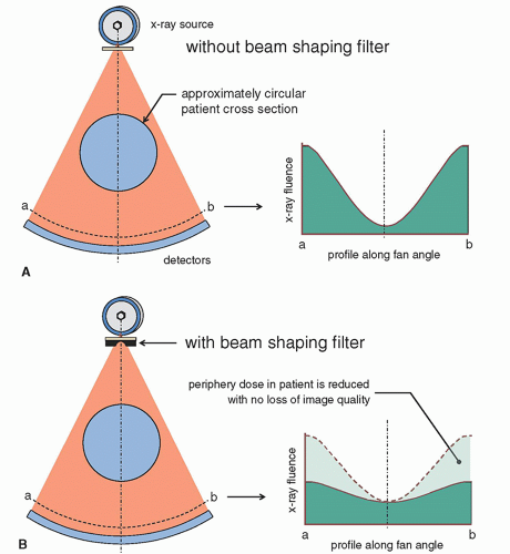▪ FIGURE 10-22 This figure shows the standard fan-beam geometry in CT, with the x-ray beam emitted from the x-ray source and then striking the detector. A. The cross section of most patients tends to be circular (bodies and heads), and in the absence of a beam shaping filter this would lead to the distribution of x-ray fluence as illustrated—with high fluence levels striking the detector at the periphery, but low fluence levels striking the detector under the center of the patient. B. A beam shaping filter, often called a bow tie filter, is positioned near the x-ray source and shapes the x-ray beam to reduce the high x-ray fluence levels at the periphery of the fan beam. The bow tie filter reduces the imbalance of signal levels received at the center and periphery of the detector, and in doing so provides considerable radiation dose reduction to the periphery of the patient—with no loss in image quality.

10.2.9 View Sampling

The bandwidth of the data acquisition chain is intrinsic to the design of a CT scanner. The view sampling of the scanner is related to both the rotation period of the gantry around 360°, and the number of samples that the detector system can acquire in this period of time (i.e., frames per second, FPS). Recalling that for most whole-body CT scanners, the x-ray tube is not pulsed, this means that the frame rate of the detector
system is a fundamental limitation to view sampling. Figure 10-24A illustrates view sampling. To illustrate the consequences of view sampling, let’s assume a simple example where the gantry rotation period is 0.5 s, and the data acquisition is 2,000 FPS. This combination of acquisition parameters results in a view sampling angle (dr) of 0.36° (1,000 views around 360°). Figure 10-24B shows that for a given view sampling angle, the width of the sampling sector increases from the center of the FOV to the periphery, as r dr. For example, for the sampling conditions described above, the width of the sampling sector is 0.31, 0.63, 0.94, and 1.26 mm at radii of 50, 100, 150, and 200 mm, respectively. The dimensions of a typical pixel in CT reconstruction with a 512 matrix range from about 0.5 to 0.7 mm for body imaging. Notice that the blurring caused by view sampling (which increases with radius in the FOV) is greater than the pixel dimensions for radii greater than 100 mm (i.e., a FOV diameter of 200 mm). While the use of x-ray focal spot dithering (Fig. 10-17) can essentially freeze the motion of the focal spot during gantry rotation, the detector array is still rotating.

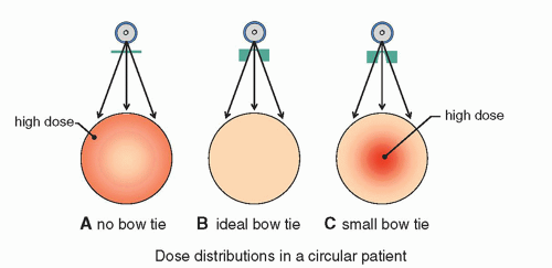▪ FIGURE 10-23 This figure illustrates the relative dose distributions between a CT system with (A) no bow tie, (B) a well-designed bow tie filter, and (C) a bow tie filter that is too centrally focused. The primary role of the bow tie filter is to reduce dose to the periphery of the patient.

▪ FIGURE 10-24 A. Most CT scanners operate the x-ray tube in continuously-on mode during CT acquisition, that is, the x-ray source is not pulsed. View sampling is defined by the data acquisition system associated with the detector arrays, which operate with relatively high bandwidth. For example, to acquire 1,000 views over 360° rotation of the gantry in 0.35 s, each detector needs to be sampled at almost 3,000 samples per second. B. This figure shows that for a given view sampling width/angle, the width of the sampling sector increases from the center of the field-of-view to the periphery, as r dr.

Only gold members can continue reading. Log In or Register to continue