X-ray Dosimetry in Projection Imaging and Computed Tomography
Radiation dosimetry is a field of study that encompasses the measurement and calculation of ionizing radiation energy deposition into matter. Dosimetric quantities and units are used in estimating radiation dose to patients, workers, and members of the public. Dosimetric quantities and units were discussed in Chapter 3. Some of these quantities, such as absorbed dose and kerma, are defined entirely in terms of other physical quantities, particularly energy and mass. Other quantities, equivalent dose, effective dose equivalent, and effective dose, are intended for use in radiation protection and involve the use of weighting factors chosen by expert bodies to account for the detriment from the biological effects of ionizing radiation. This chapter addresses the application of dosimetry to x-ray projection imaging and x-ray computed tomography.
11.1 X-RAY TRANSMISSION
Understanding x-ray dosimetry starts with an understanding of the factors in an x-ray system that lead to a specific x-ray spectrum that is incident upon the patient. This spectrum interacts with the patient’s tissues by several mechanisms that lead to radiation dose deposition in those tissues. The details of x-ray production are described in Chapter 6. A typical x-ray spectrum used in diagnostic radiology shows x-ray photon fluence as a function of x-ray energy for a tube potential of 100 kV and 3 mm inherent aluminum filtration (Fig. 11-1). The spectrum consists of bremsstrahlung radiation and tungsten characteristic radiation peaks at ˜58 and ˜67 keV and is commonly referred to as polyenergetic, indicating a range of x-ray energies.
As described in Chapter 3, x-ray interactions within the tissues of the patient have energy dependencies that must be considered for accurate radiation dosimetry. Indeed, the dose deposited by primary photons (those emitted by the x-ray tube) at a specific depth (x) within the patient is computed for each photon energy (E), and then the total dose at that depth is summed (integrated) over the entire x-ray spectrum:
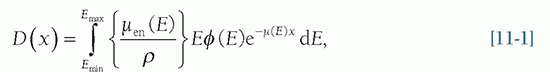
where φ (E) is the photon fluence (photons/cm2), [µen(E)/ρ] is the mass-energy absorption coefficient for photons of energy E, ρ is the density of the tissue, and µ(E) is the linear attenuation coefficient for photons of energy E. As is mentioned below, this equation does not account for energy deposition by scattered photons and so severely underestimates actual doses.
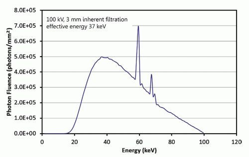 ▪ FIGURE 11-1 A typical x-ray spectrum used in radiography, fluoroscopy, and other x-ray imaging systems is illustrated. This is a 100-kV spectrum with 3 mm of inherent aluminum filtration. The area of the spectrum is normalized to 1 mGy air kerma, and the half-value layer is 3.8 mm of aluminum. The average energy is 50 keV, and the effective energy is 37 keV. |
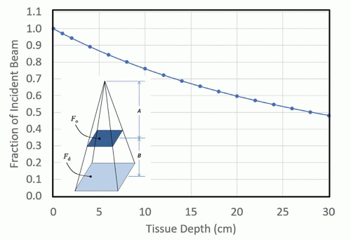
If this operation is performed for the x-ray spectrum [φ(E)] shown in Figure 11-1, using the energy-dependent linear attenuation coefficients for tissue [µ(E)], the curve marked “transmitted” is generated as shown in Figure 11-2. This curve describes the transmission of primary radiation (scatter is not included here) to the depths of a patient’s soft tissues, and the shape of the curve is due to the exponential in Equation 11-1. The curve labeled “attenuated” in Figure 11-2 illustrates the fraction of the incident beam that is attenuated (removed from the transmitted beam) due to photoelectric, Rayleigh, and Compton scattering interactions.
In most situations, the transmission of the polyenergetic x-ray spectrum through tissue can be accurately calculated using a monoenergetic approximation, as shown by the solid circles for given depths, x, in Figure 11-2. These data were computed as a single exponential:
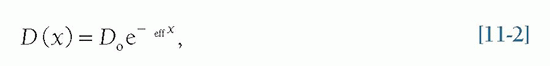
where a 37 keV monoenergetic x-ray beam was found to match the attenuation characteristics (µeff) of the 100 kV x-ray spectrum reasonably well.
As the incident x-ray beam is attenuated with depth in the patient, the diverging beam also decreases the beam intensity through the inverse square law, as illustrated in Figure 11-3. The inset on this figure demonstrates the nature of the inverse square law, with the same number of unattenuated photons passing through two different planes. The number of photons per unit area, the photon fluence, is reduced in the more distant plane because it has a larger area. Since the area increases as the square of the distance from the source, a corresponding reduction of the primary x-ray beam intensity occurs as a function of depth as shown by the curve. The x-ray dose is therefore the product of the transmission curve shown in Figure 11-2 and the inverse square law curve shown in Figure 11-3. If the beam is not divergent, which would be called a “parallel beam,” then the inverse square law is not at play. Hence, the transmission curve shown in Figure 11-2 is that of a parallel beam geometry, a common way of depiction that does not depend on a specific geometry, such as the x-ray source-to-object distance.
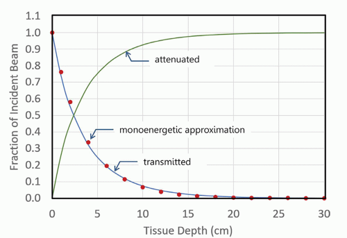 ▪ FIGURE 11-2 The transmitted x-ray beam shows the approximately exponential transmission versus tissue depth for the x-ray spectrum illustrated in Figure 11-1. The corresponding symbols demonstrate the transmission of a monoenergetic x-ray beam comprised of 37-keV x-ray photons, showing the monoenergetic approximation to the attenuation curve of the 100-kV polyenergetic spectrum. As a beam of photons passes through tissue, attenuation processes including the photoelectric effect, Rayleigh scatter, and Compton scatter occur, and these photons that have been eliminated from the primary beam are shown as the attenuated curve. The data in this curve show only the attenuation of the primary x-ray beam, assuming a parallel beam geometry. While the transmission curve appears to reach zero at about 25 cm of tissue depth, a logarithmic vertical axis would show penetration to 0.1%, 0.01%, or greater. |
 ▪ FIGURE 11-3 Because the x-ray beam is emitted from essentially a point source, the inverse square law also reduces the intensity of the beam as a function of tissue depth, even if there was no tissue present. This curve assumes a specific x-ray beam geometry, where A = SSD = 68 cm, and B = 30 cm (see inset). |
The transmission curve shown in Figure 11-2 only describes the passage of the primary beam through the tissues of the patient and does not include any tissue heterogeneity such as bones or gas pockets. In addition, when a primary x-ray photon experiences a scattering interaction, it is considered a scattered photon, and there is no simple equation to describe the actual composition of the primary and scattered photons as a function of depth. The generation of x-ray scatter and the complex geometry of the trajectory of scatter requires the use of computer-based Monte Carlo
techniques, as described in the next section, to accurately track the passage of both primary and scattered photons through the patient’s tissues.
techniques, as described in the next section, to accurately track the passage of both primary and scattered photons through the patient’s tissues.
11.2 MONTE CARLO SIMULATION
All modern x-ray dosimetry relies extensively on Monte Carlo simulation. Monte Carlo simulation requires a sophisticated computer program that tracks simulated x-ray photons as they are incident onto the patient, photon-by-photon, which potentially interact with tissue, and in some cases pass through the patient undergoing no interactions—these latter ones being the primary photons that are detected and used to form the image. However, for dosimetry, we are interested in the vast majority of photons (99.0%-99.9%) in the x-ray beam that do interact in the patient, and deposit dose through interactions including the photoelectric effect and Compton scattering.
Monte Carlo simulations are often described as computing the random walk of a photon as it interacts with the patient’s tissues, similar to that shown in Figure 11-4. Typically, this involves tracing the path of billions of x-ray photons through the object, using the computer to keep track of where energy is deposited. While this walk is stochastic in nature, it is not truly random because virtually all of the interactions between x-ray photons in the tissues in the body are described statistically, including the photoelectric effect, Rayleigh scatter, and Compton scatter. In order to include the statistical properties of x-ray scattering, all Monte Carlo routines use
random number generators. A random number generator is the equivalent of a dice roll for a computer, but uses a subroutine that returns random numbers, typically in the interval from 0 to 1; these are then used with some additional mathematics to accurately compute the stochastic physical processes that underlie the Monte Carlo simulation. Most Monte Carlo simulations include both the attenuation processes (Fig. 11-2) as well as the geometry-dependent inverse square law (Fig. 11-3). As discussed in Section 3.4, the quantity absorbed dose is defined as energy deposited by ionizing radiation per unit mass.
random number generators. A random number generator is the equivalent of a dice roll for a computer, but uses a subroutine that returns random numbers, typically in the interval from 0 to 1; these are then used with some additional mathematics to accurately compute the stochastic physical processes that underlie the Monte Carlo simulation. Most Monte Carlo simulations include both the attenuation processes (Fig. 11-2) as well as the geometry-dependent inverse square law (Fig. 11-3). As discussed in Section 3.4, the quantity absorbed dose is defined as energy deposited by ionizing radiation per unit mass.
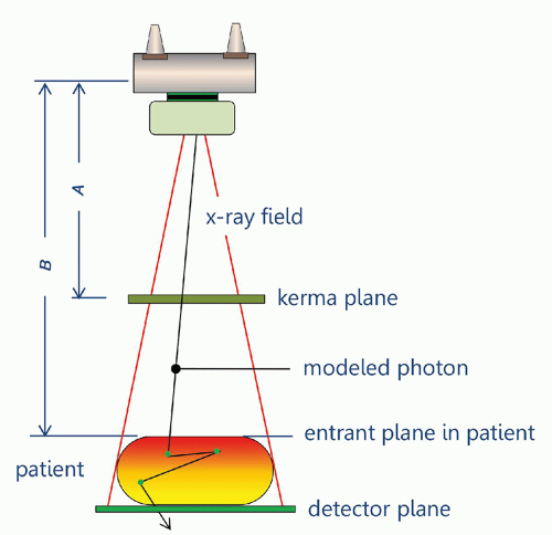 ▪ FIGURE 11-4 A typical design for Monte Carlo simulation of dose deposition is illustrated. The simulated (virtual) x-ray beam is emitted from a point source and is collimated onto a detector plane. X-ray interactions are computed in a virtual patient, where the dose deposition and its distribution are tallied. The air kerma passing through the kerma plane is recorded, and the radiation dose in the patient is also tallied. This geometry can then be used to define a coefficient, which is the ratio of patient dose to incident air kerma. More specific anatomical geometry can also tally dose to specific organs, and other interaction sites of interest. |
The probabilities of these interactions depend on the x-ray photon energy and the specific tissue in the patient, including soft tissue, adipose tissue, bone, etc. When an x-ray photon interacts via the photoelectric effect in tissue, all of the energy of that photon is deposited locally and therefore contributes to radiation dose. For high Z attenuators (iodine contrast material and metal implants are examples in the patient), x-ray fluorescence (i.e., characteristic radiation) is typically produced after a photoelectric interaction; these x-rays then carry energy away from the interaction site. However, for the low Z elements that comprise soft tissue (e.g., C, H, O, N), the fluorescent yield is essentially zero; hence the photoelectric effect results in essentially total local absorption for most soft tissues. When an x-ray photon interacts via the Rayleigh scattering mechanism, the scattered photon carries with it the same amount of energy as the incident photon, so there is no deposition of energy. Consequently, while Rayleigh scattering redirects x-ray photons, it is a zero-dose event. This does not mean, however, that a photon that was Rayleigh scattered could not undergo a subsequent interaction that does deposit energy and hence dose. Therefore, it is necessary to track Rayleigh scattered photons during a Monte Carlo simulation to accurately calculate the radiation dose distribution. When an x-ray photon experiences Compton scattering in tissue, a fraction of its energy is deposited at the interaction site contributing to the accumulation of dose, and a larger fraction of the energy remains as a scattered photon, with a deflected trajectory. The deflection angle of x-ray scatter depends on the x-ray’s energy and the effective Z of the tissue where the interaction took place, both of which are defined in probability tables developed for this purpose.
A complete Monte Carlo simulation for a specific application, such as computing the dose of an abdominal radiograph, includes looping over the range of energies (e.g., in 1 keV steps) that are present in the simulated x-ray spectrum. For example, the 100-kV x-ray spectrum illustrated in Figure 11-1 contains photons ranging from 17 to 100 keV, so each of these photon energies is simulated using millions to billions of x-rays at each (monoenergetic) energy (i.e., 84 different runs). These intermediate results are then weighted by the photon distribution in the spectrum. While Monte Carlo simulations may use many billions (109) of virtual photons in the calculation, this is far fewer than the number of x-ray photons used in an actual x-ray imaging exam. For example, an abdominal radiograph may use the 100 kV x-ray spectrum (Fig. 11-1) and 220 mAs, and would expose an image receptor of approximately 300 × 300 mm—such an examination would require about 4 × 10¹³ x-ray photons. If 106 photons required ½ minute to run in the computer for the simulations, the full simulation (4 × 10¹³) would require 38 years. Because Monte Carlo simulations are so computationally expensive, it is not practical to perform them for individual patients undergoing a common imaging procedure. Instead, published tables produced from Monte Carlo simulations are commonly used. To correct for the fact that fewer x-ray
photons are used during Monte Carlo dose simulations, the simulation geometry (Fig. 11-4) is set up to calculate both the air kerma that is incident upon the simulated patient, as well as the corresponding radiation dose deposited in the patient. In this way, coefficients can be produced that relate the radiation dose absorbed in the patient to the air kerma incident upon the patient. These coefficients can then be used with incident kerma levels measured in the real world, in order to estimate a specific patient’s absorbed dose. For radiographic and fluoroscopic procedures, the entrance air kerma at the surface of the patient is used as a normalization point. For computed tomography procedures, the air kerma at the center of rotation (isocenter) of the gantry is used as a normalization point. While the kerma plane is placed well above the “patient” in Figure 11-4, the inverse square law can be used to compute the kerma at any location in the field.
photons are used during Monte Carlo dose simulations, the simulation geometry (Fig. 11-4) is set up to calculate both the air kerma that is incident upon the simulated patient, as well as the corresponding radiation dose deposited in the patient. In this way, coefficients can be produced that relate the radiation dose absorbed in the patient to the air kerma incident upon the patient. These coefficients can then be used with incident kerma levels measured in the real world, in order to estimate a specific patient’s absorbed dose. For radiographic and fluoroscopic procedures, the entrance air kerma at the surface of the patient is used as a normalization point. For computed tomography procedures, the air kerma at the center of rotation (isocenter) of the gantry is used as a normalization point. While the kerma plane is placed well above the “patient” in Figure 11-4, the inverse square law can be used to compute the kerma at any location in the field.
In the early days of Monte Carlo simulations, mathematical phantoms comprised of simple geometrical shapes were used to simulate the geometry of the human body (Fig. 11-5A). More recently, whole-body CT images have been used to model the geometry of the human body (Fig. 11-5B). Typically, these whole-body CT scans (often produced from cadavers) are segmented into relatively large (e.g., 2 × 2 × 2 mm, 5 × 5 × 5 mm, etc.) voxels for use in Monte Carlo simulations. Once a mathematical model of the patient is developed, specific radiographic projections or other imaging geometries need to be defined so that the radiation dose coefficients can be computed for specific clinical examinations, such as PA chest radiography, lateral head radiography, abdominal CT with helical acquisition, etc. The geometry of a PA abdominal radiograph is demonstrated in Figure 11-5A, corresponding to a 300 mm × 300 mm field of view projected onto a mathematical anthropomorphic phantom.
11.3 THE PHYSICS OF X-RAY DOSE DEPOSITION
X-rays deposit energy (and hence dose) through interactions with electrons. Both the photoelectric effect and Compton scattering interactions ionize an atom or molecule at the site of interaction, resulting in the ejection of an energetic electron. These
energetic electrons interact with tissue, depositing most of their energy in a very small volume. Indeed, the initial electron ejected from an x-ray interaction will collide with many other electrons in atoms and molecules before it comes to rest, causing subsequent ionization events along its path. These secondary energetic electrons (called “delta rays”) impart much of the radiation energy near the initial ionization event. This energy deposition causes chemical changes that damage molecules of biological importance. The ultimate health impact of this molecular damage will depend on which molecules have been damaged, the extent of the damage, the subsequent fidelity of repair processes, as well as many other factors discussed in greater detail in Chapter 20. DNA is, of course, a critical molecule, and radiation-induced DNA base damage and double-strand breaks followed by base excision repair and nonhomologous end-joining, respectively, are well-known examples of these ubiquitous damage and repair processes occurring throughout life.
energetic electrons interact with tissue, depositing most of their energy in a very small volume. Indeed, the initial electron ejected from an x-ray interaction will collide with many other electrons in atoms and molecules before it comes to rest, causing subsequent ionization events along its path. These secondary energetic electrons (called “delta rays”) impart much of the radiation energy near the initial ionization event. This energy deposition causes chemical changes that damage molecules of biological importance. The ultimate health impact of this molecular damage will depend on which molecules have been damaged, the extent of the damage, the subsequent fidelity of repair processes, as well as many other factors discussed in greater detail in Chapter 20. DNA is, of course, a critical molecule, and radiation-induced DNA base damage and double-strand breaks followed by base excision repair and nonhomologous end-joining, respectively, are well-known examples of these ubiquitous damage and repair processes occurring throughout life.
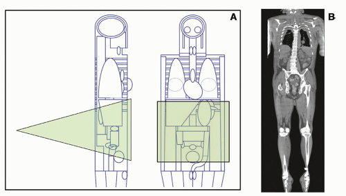 ▪ FIGURE 11-5 A. Historically, Monte Carlo studies made use of anatomical models defined by simple geometrical shapes; here the Medical Internal Radiation Dose (MIRD) phantom is illustrated. B. The power of modern computers combined with the availability of high-resolution anatomical data from CT scans have allowed Monte Carlo simulations to be performed with very detailed anatomical models. |
Figure 11-6 illustrates the concept of air kerma. “Kerma” stands for K inetic Energy Released in Matter and was discussed in Chapter 3. X-ray photons entering a small volume of air interact with the air molecules, whereby each interaction produces an ion pair—an energetic electron and the positively charged atom or molecule that it came from. Normally the accurate measurement of radiation assumes that within the measurement volume of air, the energy carried out of the volume by electrons leaving the volume is equal to the energy carried into the volume by electrons produced outside of the volume—so-called electron equilibrium. Kinetic energy is the energy of motion, and it is these energetic electrons (primarily) that ultimately produce absorbed dose. Kerma (K) is defined as a “point quantity,” although the energy considered is transferred to electrons in a very small mass of material. The sum of this kinetic energy (in joules), divided by the mass (in kilograms) of air in the measurement volume is the air kerma, with the typical unit of milligray (mGy) in diagnostic radiology.
Energetic electrons can graze an air molecule (e.g., O2 or N2) and experience the nuclear charge of an atom, causing the electron to be decelerated. As described in Chapter 6, when electrons bombard a target inside the x-ray tube,
they are decelerated and produce bremsstrahlung radiation. The same interaction can occur in the volume of air, generating a bremsstrahlung x-ray that then leaves the volume of air, taking with it some of the kinetic energy (Er, r = radiative) that was originally transferred to the electron (Fig. 11-7). The remaining absorbed energy (Een) in the volume of air is the difference between the initial energy transferred to electron motion (Etr, tr = transferred), subtracting the loss of energy through radiative emission:
they are decelerated and produce bremsstrahlung radiation. The same interaction can occur in the volume of air, generating a bremsstrahlung x-ray that then leaves the volume of air, taking with it some of the kinetic energy (Er, r = radiative) that was originally transferred to the electron (Fig. 11-7). The remaining absorbed energy (Een) in the volume of air is the difference between the initial energy transferred to electron motion (Etr, tr = transferred), subtracting the loss of energy through radiative emission:
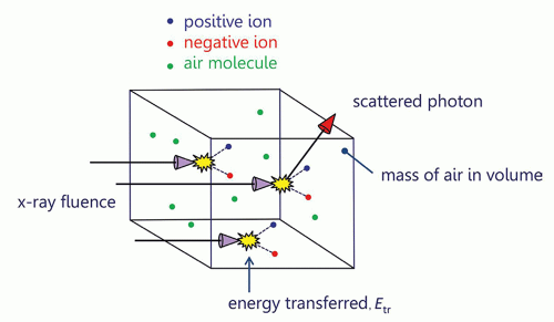 ▪ FIGURE 11-6 The basic concept of air kerma is illustrated. X-rays are incident upon a small volume of air and ionize air atoms producing ion pairs as defined in the figure. With these interactions, x-ray photons transfer their energy to the ion pair, resulting in kinetic energy of these charged particles. When a Compton scattering event takes place, the scattered photon leaves the volume of interest. The air kerma (kinetic energy released in matter) is the energy transferred to charged particles, divided by the mass of the air in the measurement volume. |
It is the absorbed energy Een (in joules) per unit mass of the volume (in kilograms) that gives rise to the absorbed dose. Figure 11-8 illustrates the absorbed dose, and if in a volume of air, this would be the air dose. The amount of bremsstrahlung radiation released (Fig. 11-7) in the diagnostic x-ray energy region is very low—almost to the point of being negligible. However, for x-rays with higher energies (>250 keV) the radiative emission (Er) can be a larger fraction of Etr. So in the diagnostic energy region, Er → 0, and thus Etr ≈ Een, meaning that air kerma is about equal to air dose in diagnostic radiology.
It was stated above that the volume shown in Figure 11-8 could be air, but this volume could just as well be tissue—the mechanisms of radiation dose deposition that occur in a volume of low-density air are the same that occur in a small volume of near unit-density tissue. The description above discusses the physics of dose deposition, and also describes some of the elements that a Monte Carlo simulation program must take into consideration in order to perform a radiation dose calculation (in silico).
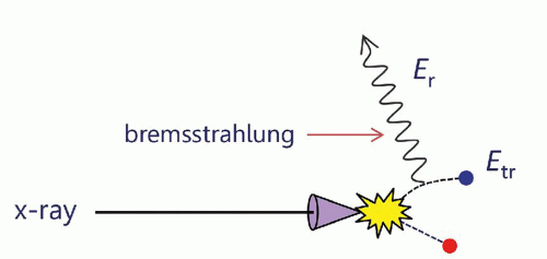 ▪ FIGURE 11-7 When an x-ray interacts with an atom or molecule that transfers energy to an ion pair (Etr), subsequent interactions between an energetic electron and other atoms in the interaction volume can result in deceleration of the electron, producing bremsstrahlung radiation (Er: radiated energy). When the bremsstrah-lung x-ray leaves the measurement volume, the absorbed energy (Een) is given by: Een = Etr – Etr. |
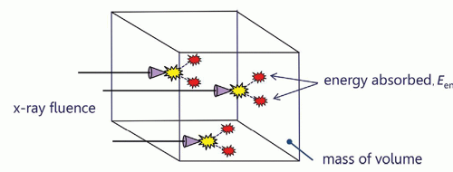 ▪ FIGURE 11-8 When x-ray photons (x-ray fluence) are incident upon the measurement volume, initially energy is transferred (Etr), some energy may be radiated away (as shown in Fig. 11-7), and the energy that remains Een, divided by the mass of that volume, represents the absorbed dose. The volume of interest in this figure could be filled with air, and hence the dose would be the air dose; however, this can also be a small volume of tissue, corresponding to the absorbed dose in tissue. |
11.4 DOSE METRICS
The concept of radiation dose has evolved considerably as our understanding of the effects of ionizing radiation has advanced; consequently, there are a number of metrics that describe radiation dose in different ways. Each of these metrics has utility in describing and understanding radiation dose from x-ray diagnostic medical imaging procedures. Radiation dose in nuclear medicine procedures is described in Chapter 16. It is important to note that, as we review different quantities that describe radiation dose, in some cases (but not all) the unit associated with a quantity may change. It is very important to understand the differences between the quantities and the units and to make sure that the proper unit is used when discussing the associated quantity.
11.4.1 Entrance Skin Air Kerma
The entrance skin air kerma (ESAK) simply describes the amount of radiation incident upon the surface of the patient (formerly the quantity entrance skin exposure was used). For radiographic procedures using x-ray beams with similar energy spectra, ESAK is roughly proportional to the surface dose in the patient and so can be used to compare procedures from a dosimetric perspective. ESAK is an appropriate metric for radiographic (including mammographic) and fluoroscopic procedures, but not for computed tomography. The ESAK is typically estimated free-in-air, (i.e., neglecting scatter from the patient) and can be determined from the known output characteristics of the x-ray system in association with the geometry of the radiographic procedure (discussed below).
Imagine a radiographic procedure of a patient’s abdomen, where the surface of the patient’s abdomen is located 70 cm from the x-ray source. By measuring the output of the system at 70 cm from the x-ray source using a radiation meter and ionization chamber with no other object in the field of view, the air kerma “free-in-air” is determined. However, if the patient (or more likely a phantom) is positioned at 70.1 cm from the x-ray source and the ionization chamber is positioned just in front of the phantom with the same x-ray exposure settings (i.e., kV, mA, exposure time), the radiation meter will record a larger value of air kerma by about 15%-20%, because scattered radiation coming back from the phantom will be detected, in addition to the primary radiation emanating from the x-ray tube. So, when ESAK is used as a dose metric unless otherwise stipulated, this measurement is made in the absence of a phantom and therefore in the absence of backscattered radiation, in the geometry known as “free-in-air.” For air kerma measured at the entrant surface of the skin, the common unit for this measurement value is mGy.
11.4.2 Entrance Skin Dose
As the x-ray beam enters the first microscopic layers of the skin, the radiation dose imparted to that layer of skin is referred to as the entrance skin dose. Recall that from Figure 11-8, in diagnostic radiology the air kerma is essentially equal to the air dose, and thus the air dose just above the layer of skin is equivalent numerically (both typically in the units of mGy) to the air kerma, as Dair  Kair. When considering only the dose to a microscopic layer of skin or tissue at the surface of the patient, two things are intentionally neglected: (1) the attenuation that occurs at depth in the tissue, and
(2) backscattered radiation that would contribute to the dose at the entrant surface. With this understanding, the dose to the entrance skin (tissue) is computed as:
Kair. When considering only the dose to a microscopic layer of skin or tissue at the surface of the patient, two things are intentionally neglected: (1) the attenuation that occurs at depth in the tissue, and (2) backscattered radiation that would contribute to the dose at the entrant surface. With this understanding, the dose to the entrance skin (tissue) is computed as:
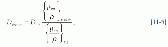
where the ratio of the mass-energy attenuation coefficients (tissue over air) is used to convert the air dose to the entrance surface to tissue dose. Except for bone, the ratio of mass-energy attenuation coefficients for soft tissues in Equation 11-5 is approximately 1.09.
11.4.3 Absorbed Dose
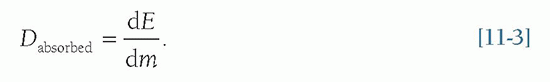
The quantity absorbed dose embodies the fundamental concept of radiation dose, with its strengths and weaknesses. Fundamentally, absorbed dose is defined as  , i.e., energy per unit mass (Eq. 11-3). When the energy is expressed in joules, and the mass is expressed in kilograms, the absorbed dose takes on the unit gray. Strictly speaking, absorbed dose is defined at a specific point, and the dose nearly always varies with location in a phantom or patient. For x-ray beams used in diagnostic and interventional imaging, the dose is higher in the tissues closer to the source than those deeper in the body. The average (mean) absorbed dose is what is often referred to when the simple term “dose” is used. Given this definition, the quantity absorbed dose in the context of biological risk is all too often open to misinterpretation, due to a number of factors including the volume of tissue that received the dose, and the specific tissue that received the dose. For example, which is more concerning from a radiation risk perspective? (1) An average dose of 10 Gy to your finger, or (2) an average dose of 10 mGy to your abdomen? Example 1 results in a total energy imparted of 0.2 joules (J) deposited in a 20-g finger, and example 2 results in 0.2 J deposited in a 20-kg abdomen. So, without specifying the total mass of tissue that receives a given absorbed dose value, the associated radiation risk is hard to assess. In addition, the organ or tissue in which the dose is deposited also affects the risk.
, i.e., energy per unit mass (Eq. 11-3). When the energy is expressed in joules, and the mass is expressed in kilograms, the absorbed dose takes on the unit gray. Strictly speaking, absorbed dose is defined at a specific point, and the dose nearly always varies with location in a phantom or patient. For x-ray beams used in diagnostic and interventional imaging, the dose is higher in the tissues closer to the source than those deeper in the body. The average (mean) absorbed dose is what is often referred to when the simple term “dose” is used. Given this definition, the quantity absorbed dose in the context of biological risk is all too often open to misinterpretation, due to a number of factors including the volume of tissue that received the dose, and the specific tissue that received the dose. For example, which is more concerning from a radiation risk perspective? (1) An average dose of 10 Gy to your finger, or (2) an average dose of 10 mGy to your abdomen? Example 1 results in a total energy imparted of 0.2 joules (J) deposited in a 20-g finger, and example 2 results in 0.2 J deposited in a 20-kg abdomen. So, without specifying the total mass of tissue that receives a given absorbed dose value, the associated radiation risk is hard to assess. In addition, the organ or tissue in which the dose is deposited also affects the risk.To add to the complication of using dose to convey risk, when a patient has had multiple diagnostic medical imaging procedures, for example after trauma, there is no single number that conveys risk. If a patient received 70 mGy to the head, 1.2 mGy to the knee, and 10 mGy to the abdomen after an automobile injury, there is no simple way to use absorbed dose as a metric to quantify this. That said, absorbed dose—or just “dose”—is the gold standard measurement describing one or more radiation exposure events.
11.4.4 Mean Glandular Dose
While the absorbed dose is the most appropriate metric for describing the magnitude of radiation exposure to a patient’s organs, radiation exposure to the breast has a unique metric. The breast is comprised of several tissues, including fibroglandular tissue, adipose tissue (fat), and skin. However, the radiosensitivity of the glandular tissue for future cancer is far greater than that of the skin or adipose tissue. Indeed,
breast cancer refers to cancers of the glandular tissues in the breast, not the adipose or skin tissues. Consequently, and specific to breast imaging, the mean glandular dose (MGD, also referred to as the mean fibroglandular dose) is the preferred metric for estimating radiation dose in the breast. Hence, the Monte Carlo routines that are used for computing dosimetry in breast imaging specifically tabulate the radiation dose delivered to the glandular tissue. The unique dosimetry used for mammography is discussed in Chapter 8.
breast cancer refers to cancers of the glandular tissues in the breast, not the adipose or skin tissues. Consequently, and specific to breast imaging, the mean glandular dose (MGD, also referred to as the mean fibroglandular dose) is the preferred metric for estimating radiation dose in the breast. Hence, the Monte Carlo routines that are used for computing dosimetry in breast imaging specifically tabulate the radiation dose delivered to the glandular tissue. The unique dosimetry used for mammography is discussed in Chapter 8.
11.4.5 Organ Dose
Metrics
The metric commonly used for evaluating the dose to an organ or tissue with regard to possible stochastic effects is the average (mean) absorbed dose delivered to the specific organ or tissue. It may be calculated as the quotient E/m, where E is the total energy imparted in the organ or tissue and m is the mass of the organ or tissue. The volume of interest in which the imparted energy (E) and mass (m) are computed is defined by the organ boundaries. For paired organs such as breasts and kidneys, the organ volume includes both organs. Calculating mean organ doses is the first (and likely most important) step in estimating risk of stochastic effects such as cancer from medical imaging procedures using ionizing radiation. Mean organ doses are unique because the mass of the entire organ is used in the calculation (m), even if only a fraction of the organ was exposed to radiation. For example, for a 10-kg liver, if 40% of the liver volume experienced an x-ray imaging procedure (such as a lesion-targeted CT scan) that deposited a total of 0.10 J in the liver, the mean organ dose to the liver would be 0.10 J/10 kg = 0.01 Gy or 10 mGy. Had the entire liver been exposed at the same radiation levels, the energy deposited would have been 0.25 J and the mean organ dose would have been 25 mGy. If a targeted radiographic procedure exposed the left kidney to 0.20 mGy, and the right kidney received no appreciable radiation, the mean kidney organ dose would be 0.10 mGy. The implicit assumption in the methodology just described is that at low dose, the stochastic risk (e.g., future cancer in the exposed organ) is the same whether one half of the organ receives all of the radiation or if the exposure was evenly distributed throughout the entire organ.
Anthropomorphic Phantoms
With well-defined patient anatomy in the form of an anthropomorphic phantom incorporated into computer code, the organ doses resulting from x-ray exposure can be estimated using Monte Carlo techniques. The original anthropomorphic phantoms used with Monte Carlo programs to calculate radiation dose in the late 1950s and early 1960s employed rather elementary shapes like cylinders, spheres, ellipsoids, and prolate spheroids due to the lack of computational power available to the scientists of that era. Stylized computational phantoms have had a long history of development. In the 1960s much of the effort was tied to the need to estimate the absorbed dose to organs in patients who had been administered radiopharmaceuticals in the rapidly developing field of nuclear medicine and to radiation workers who may have become internally contaminated with radioactive material. Figure 11-9A shows organ doses (as different colors) using a 1980s era anthropomorphic phantom for a typical x-ray imaging procedure of the upper abdomen and thorax, with the different colors representing different organ doses. The organ and body contours of these stylized phantoms were defined by 3D mathematical surface equations. Further refinements led to CT based voxel Monte Carlo simulations of phantoms in which organs and body tissues were defined by groupings of 3-D cuboids or voxels
to define the anatomical structures based on segmentation of patient medical images. While these phantoms were anatomically very accurate, they were not very flexible (with regard to adjustments for desired changes in resolution or age or body habitus of the phantom) and were computationally intensive. The optimal balance between accuracy and simulation efficiency came in the form of hybrid modeling. The hybrid modeling of the imaging processes combines the analytical and Monte Carlo simulation methods as well as the ability to integrate different Monte Carlo packages. Modern computational phantoms are typically constructed by the hybrid method defining surfaces or meshes based on the segmentation of 3-D patient imaging data (e.g., MRI and CT). The PHANTOMS library developed from CT images of patients shown in Figure 11-9B is an example of employing the hybrid method and was the product of a collaboration between the University of Florida and the National Cancer Institute (Geyer et al., 2014; Lee et al., 2010). Best quality anatomical reference CT images were selected from an archive of 1,000+ patients. More than 100 organs and tissues were manually segmented and reviewed by practicing radiologists. The original PHANTOMS library consisted of a series of reference male and female anatomies (newborn, 1-, 51-, 10-, 15-year-old, and adult). This library was later extended to 370 phantoms representing children and adults of both genders and various heights and weights, Figure 11-9C. NCI researchers also added anatomical details such as
lymphatic nodes, substructures of the heart (e.g., atria, ventricles, arteries), and substructures of the brain (e.g., gray and white matter, cerebellum, brain stem). The PHANTOMS library was carefully adjusted to match several international reference data including reference person height and weight, organ mass, tissue elemental composition, and dimensions of gastrointestinal structures. The pediatric phantoms have been adopted by the International Commission on Radiological Protection (ICRP) as an international reference (ICRP, 2020[q]).
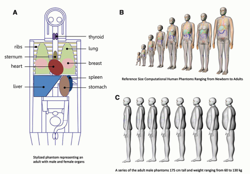 ▪ FIGURE 11-9 The x-ray interactions illustrated in Figures 11-6 to 11-8 show fundamental interactions that take place physically, but in Monte Carlo modeling these interactions are calculated mathematically, with the statistically known x-ray cross sections, attenuation coefficients, and scattering angles within an anthropomorphic phantom to estimate absorbed dose. (A) represents a 1980s stylized anthropomorphic phantom developed at Oak Ridge National Laboratory representing adult with male and female anatomy while (B) is an example of state-of-the-art (2020) hybrid phantoms from the National Cancer Institute’s library of computational human phantoms showing their reference size computational human phantoms ranging from newborn to male and female adults and (C) their series of the adult male phantoms 175 cm tall of varying body habitus with weight ranging from 60 to 130 kg. (B: Reprinted with permission from the National Cancer Institute: Division of Cancer Epidemiology and Genetics. https://ncidose.cancer.gov/#phantoms. Accessed July 6, 2020. C: Reproduced with permission from Chang LA, Borrego D, Lee C. Body-weight dependent dose coefficients for adults exposed to idealised external photon fields. J Radiol Prot. 2018;38(4):1441. © IOP Publishing. All rights reserved.) |
No One Dose Metric Can Do It All
It is often said that a tally of organ doses represents the most comprehensive assessment of radiation dose from medical imaging procedures; however, there is no single metric that quantifies this. This is because the detriment of radiation exposure to the different organs has been studied in detail. Early classical cell survival studies demonstrated that for a given absorbed dose to the same type of cells in culture, some forms of radiation (like doubly charged alpha particles that produce dense ionization tracks) produced more cell death than sparsely ionizing forms of radiation (like x- and γ-ray and beta particles). Furthermore, based on the studies of radiation exposures to large populations (primarily the Japanese A-bomb survivors), it is known that different organs demonstrate different radiosensitivity with respect to developing radiogenic cancers. The ICRP developed the quantities equivalent dose (H) and effective dose (E) to take these and other factors (discussed in Chapter 21), relevant to the potential of future risks to a population exposed to low dose radiation.
Equivalent Dose
As mentioned in Chapter 3, the ICRP established the radiation weighting factors (wR) to account for the greater effectiveness of higher Linear Energy Transfer (LET) radiations for producing biologic damage compared to low LET radiation (x-rays, γ rays, and energetic electrons). Low LET radiation is assigned a wR value of 1. Higher LET radiations, such as protons and alpha particles, are assigned wR values greater than 1 (e.g., alpha wR = 20) reflecting the fact that the damage caused by the dense ionization tracks of this type of radiation are more difficult to repair per unit dose than the more sparsely ionizing low LET radiations. When the absorbed dose is multiplied by the appropriate radiation weighting factor, it is transformed from a physical quantity (i.e., energy per unit mass) to a radiation protection quantity equivalent dose (H):
While the equivalent dose is numerically equal to the absorbed dose for x-rays, since wR = 1, it should be kept in mind that the equivalent dose is a different quantity (with the unit of a sievert, Sv) than the absorbed dose (with the unit of Gy).
11.4.6 Effective Dose
The first thing to know about effective dose is that, like the equivalent dose, it is not a dose in the true sense of the word. Rather, the effective dose is a radiation protection quantity that incorporates a rough approximation of the relative biological variations in tissue sensitivities by assigning particular organs and tissue (T) the proportion of the detriment (harm) from stochastic effects (e.g., cancer, hereditary and other effects discussed further in Chapter 20) resulting from irradiation of that tissue compared to uniform whole-body irradiation. The proportion of the total (i.e., 1.0) assigned to a particular organ/tissue is referred to as the tissue weighting factor (wt). Tissue weighting factors range from wt = 0.01 for radioresistant tissues (e.g., brain), to wt = 0.12 for
more radiosensitive tissues such as the intestines, lung, breast, stomach, and bone marrow (Table 11-1). In assigning the tissue weighting factors, the ICRP relied primarily on the results of epidemiological studies on large human populations exposed to radiation with long-term follow-up, to assess the relative risk of radiation-induced cancer (and other less frequent bioeffects) for each organ or tissue type.
more radiosensitive tissues such as the intestines, lung, breast, stomach, and bone marrow (Table 11-1). In assigning the tissue weighting factors, the ICRP relied primarily on the results of epidemiological studies on large human populations exposed to radiation with long-term follow-up, to assess the relative risk of radiation-induced cancer (and other less frequent bioeffects) for each organ or tissue type.
Related posts:
Stay updated, free articles. Join our Telegram channel

Full access? Get Clinical Tree


