Magnetic Resonance Basics: Magnetic Fields, Nuclear Magnetic Characteristics, Tissue Contrast, Image Acquisition


Magnetic Resonance Basics: Magnetic Fields, Nuclear Magnetic Characteristics, Tissue Contrast, Image Acquisition


Nuclear magnetic resonance (NMR) is the spectroscopic study of the magnetic properties of the nucleus of the atom. The protons and neutrons of the nucleus have a magnetic field associated with their nuclear spin and charge distribution. Resonance is an energy coupling that causes the individual nuclei, when placed in a strong external magnetic field, to selectively absorb, and later release, energy unique to those nuclei and their surrounding environment. The detection and analysis of the NMR signal has been extensively studied since the 1940s as an analytic tool in chemistry and biochemistry research. NMR is not an imaging technique but rather a method to provide spectroscopic data concerning a sample placed in a small volume, high field strength magnetic device. In the early 1970s, it was realized that magnetic field gradients could be used to localize the NMR signal and to generate images that display magnetic properties of the proton, reflecting clinically relevant information, coupled with technological advances and development of “body-size” magnets. As clinical imaging applications increased in the mid-1980s, the “nuclear” connotation was dropped, and magnetic resonance imaging (MRI), with a plethora of associated acronyms, became commonly accepted in the medical community.

MR applications continue to expand clinical relevance with higher field strength magnets, improvements in anatomic and physiologic data acquisition/analysis, and advances in spectroscopy for accurate electronic tissue biopsies. The high contrast sensitivity to soft tissue differences and the inherent safety to the patient resulting from the use of non-ionizing radiation have been key reasons why MRI has supplanted many CT and projection radiography methods. With continuous improvements in image quality, acquisition methods, and equipment design, MRI is often the modality of choice to examine anatomic and physiologic properties of the patient. There are drawbacks, however, including high equipment and siting costs, scan acquisition complexity, relatively long imaging times, significant image artifacts, patient claustrophobia, and MR safety concerns.

This chapter reviews the basic properties of magnetism, concepts of resonance, tissue magnetization and relaxation events, generation of image contrast, and basic methods of acquiring image data. Advanced pulse sequences, illustration of image characteristics/artifacts, MR spectroscopy (MRS), MR safety, and biologic effects are discussed in Chapter 13.


12.1 MAGNETISM, MAGNETIC FIELDS, AND MAGNETIC PROPERTIES OF MATERIALS


12.1.1 Magnetism

Magnetism is a fundamental property of matter; it is generated by moving charges, usually electrons. Magnetic properties of materials result from the organization and motion of the electrons in either a random or a nonrandom alignment of magnetic “domains,” which are the smallest entities of magnetism. Atoms and molecules have electron orbitals that can be paired (an even number of electrons cancels the magnetic field) or unpaired (the magnetic field is present). Most materials do not exhibit overt magnetic properties, but one notable exception is the permanent magnet, in which the individual magnetic domains are aligned in one direction.

Unlike the monopole electric charges from which they are derived, magnetic fields exist as dipoles, where the north pole is the origin of the magnetic field lines and the south pole is the return (Fig. 12-1A). One pole cannot exist without the other. As with electric charges, “like” magnetic poles repel and “opposite” poles attract. Magnetic field strength, B (also called the magnetic flux density), can be conceptualized as the number of magnetic lines of force per unit area, which decreases roughly as the inverse square of the distance from the source. The SI unit for B is the Tesla (T). As a benchmark, the earth’s magnetic field is about 1/20,000 = 0.00005 T = 0.05 mT. An alternate (historical) unit is the gauss (G), where 1 T = 10,000 G.


12.1.2 Magnetic Fields

Magnetic fields can be induced by a moving charge in a wire (e.g., see the section on transformers in Chapter 6). The direction of the magnetic field depends on the sign and the direction of the charge in the wire, as described by the “right hand rule”: The fingers point in the direction of the magnetic field when the thumb points in the direction of a moving positive charge (i.e., opposite to the direction of electron movement). Wrapping the current-carrying wire many times in a coil causes a superimposition of the magnetic fields, augmenting the overall strength of the magnetic field
inside the coil, with a rapid falloff of field strength outside the coil (see Fig. 12-1B). Amplitude of the current in the coil determines the overall magnitude of the magnetic field strength. The magnetic field lines extending beyond the concentrated field are known as fringe fields.
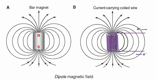


FIGURE 12-1 A. The magnetic field has two poles with magnetic field lines emerging from the north pole (N), and returning to the south pole (S), as illustrated by a simple bar magnet. B. A coiled wire carrying an electric current produces a magnetic field with characteristics similar to a bar magnet. Magnetic field strength and field density are dependent on the amplitude of the current and the number of coil turns.


12.1.3 Magnetic Properties of Materials

Magnetic susceptibility describes the extent to which a material becomes magnetized when placed in a magnetic field. In some materials, induced internal magnetization opposes the external magnetic field and lowers the local magnetic field surrounding the material. On the other hand, the internal magnetization can form in the same direction as the applied magnetic field and increase the local magnetic field. Three categories of susceptibility are defined: diamagnetic, paramagnetic, and ferromagnetic, based upon the arrangement of electrons in the atomic or molecular structure. Diamagnetic elements and materials have slightly negative susceptibility and oppose the applied magnetic field, because of paired electrons in the surrounding electron orbitals. Examples of diamagnetic materials are calcium, water, and most organic materials (chiefly owing to the diamagnetic characteristics of carbon and hydrogen molecules). Paramagnetic materials, with unpaired electrons, have slightly positive susceptibility and enhance the local magnetic field, but they have no measurable self-magnetism. Examples of paramagnetic materials are molecular oxygen (O2), deoxyhemoglobin, some blood degradation products such as methemoglobin, and gadolinium-based contrast agents. Locally, these diamagnetic and paramagnetic agents will deplete or augment the local magnetic field (Fig. 12-2), affecting MR images in known, unknown, and sometimes unexpected ways. Ferromagnetic materials are “superparamagnetic”—that is, they augment the external magnetic field substantially. These materials, containing iron, cobalt, and nickel, exhibit “self-magnetism” in many cases, and can significantly distort the acquired signals.


12.1.4 Magnetic Characteristics of the Nucleus

The nucleus, comprising protons and neutrons with characteristics listed in Table 12-1, exhibits magnetic characteristics on a much smaller scale than for atoms/molecules and their associated electron distributions. Magnetic properties are influenced by spin and charge distributions intrinsic to the proton and neutron. A magnetic
dipole is created for the proton, with a positive charge equal to the electron charge but of opposite sign, due to nuclear “spin.” Overall, the neutron is electrically uncharged, but subnuclear charge inhomogeneities and an associated nuclear spin result in a magnetic field of opposite direction and approximately the same strength as the proton. Magnetic characteristics of the nucleus are described by the nuclear magnetic moment, represented as a vector indicating magnitude and direction. For a given nucleus, the nuclear magnetic moment is determined through the pairing of the constituent protons and neutrons. If the sum of the number of protons (P) and number of neutrons (N) in the nucleus is even, the nuclear magnetic moment is essentially zero. However, if N is even and P is odd, or N is odd and P is even, the resultant non-integer nuclear spin generates a nuclear magnetic moment. A single nucleus does not generate a large enough nuclear magnetic moment to be observable, but the conglomeration of large numbers of nuclei (˜1015) arranged in a non-random orientation generates an observable nuclear magnetic moment of the sample, from which the MRI signals are derived.
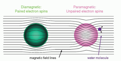


FIGURE 12-2 The local magnetic field can be changed in the presence of diamagnetic (depletion) and paramagnetic (augmentation) materials, with an impact on the signals generated from nearby signal sources such as the hydrogen atoms in water molecules.


TABLE 12-1 PROPERTIES OF THE NEUTRON AND PROTON


CHARACTERISTIC


NEUTRON


PROTON


Mass (kg)


1.674 × 10⁻²⁷


1.672 × 10⁻²⁷


Charge (coulomb)


0


1.602 × 10⁻¹⁹


Spin quantum number


½


½


Magnetic moment (J/T)


-9.66 × 10⁻²⁷


1.41 × 10⁻²⁶


Magnetic moment (nuclear magneton)


-1.91


2.79


12.1.5 Nuclear Magnetic Characteristics of the Elements

Biologically relevant elements that are candidates for producing MR signals are listed in Table 12-2. Key features include the strength of the nuclear magnetic moment, the physiologic concentration, and the isotopic abundance. Hydrogen, having the largest magnetic moment and greatest abundance, chiefly in water and fat, is by far the best element for general clinical utility. Other elements are orders of magnitude less sensitive. Of these, 23Na and 31P have been used for imaging in limited situations, despite their relatively low sensitivity. Therefore, the nucleus of the hydrogen atom, the proton, is the principal focus for generating MR signals.


12.1.6 Magnetic Characteristics of the Proton

The spinning proton or “spin” (spin and proton are used synonymously herein) is classically considered to be a tiny bar magnet with north and south poles, even though the magnetic moment of a single proton is undetectable. Large numbers of unbound hydrogen atoms in water and fat, those unconstrained by molecular bonds in complex macromolecules within tissues, have a random orientation of their protons (nuclear magnetic moments) due to thermal energy. As a result, there is no observable magnetization of the sample (Fig. 12-3A). However, when placed in a strong static magnetic field, B0, magnetic forces cause the protons to realign with the applied field in parallel and antiparallel directions with an excess of a few more oriented parallel to the B0 field (Fig. 12-3B). At 1.0 T, the number of excess protons in the parallel (low-energy state) is approximately 3 protons per million (3 × 10⁻⁶) at physiologic temperatures. Although this number seems insignificant, for a typical voxel volume in MRI, there

are about 1021 protons, so there are approximately 3 × 10-6 × 1021, or 3 × 10¹⁵, more protons in the parallel direction! This number of excess protons produces an observable “sample” nuclear magnetic moment, initially aligned with the direction of the applied magnetic field. The classical description deals with a single net magnetization of an ensemble of nuclei.


TABLE 12-2 MAGNETIC RESONANCE PROPERTIES OF MEDICALLY USEFUL NUCLEI
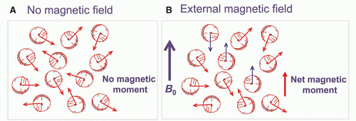


NUCLEUS


SPIN QUANTUM NUMBER


% ISOTOPIC ABUNDANCE


MAGNETIC MOMENTa


% RELATIVE ELEMENTAL ABUNDANCEb


RELATIVE SENSITIVITY


GYRO-MAGNETIC RATIO, γ/2π (MHz/T)


1H


½


99.98


2.79


10


1


42.58


3He


½


0.00014


-2.13


0


32.43


13C


0.011


0.70


18


10.71


17O


5/2


0.04


-1.89


65


9 × 10⁻⁶


5.77


19F


½


100


2.63


<0.01


3 × 10⁻⁸


40.05


23Na


3/2


100


2.22


0.1


1 × 10⁻⁴


11.26


31P


½


100


1.13


1.2


6 × 10⁻⁵


17.24


a Moment in nuclear magneton units = 5.05 × 10⁻²⁷ J/T.

b Note: by mass in the human body (all isotopes).


FIGURE 12-3 Simplified distributions of “free” protons without and with an external magnetic field are shown. A. Without an external magnetic field, a group of protons assumes a random orientation of magnetic moments, producing an overall magnetic moment of zero. B. Under the influence of an external magnetic field, some protons (blue vectors) in the tissue occupy two spin states: parallel or antiparallel to B0. The difference in number of spins between these two states is a few per million. A slightly greater number exist in the parallel direction at equilibrium, resulting in a measurable net magnetic moment of the tissue sample in the direction of B0.
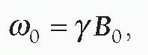
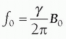
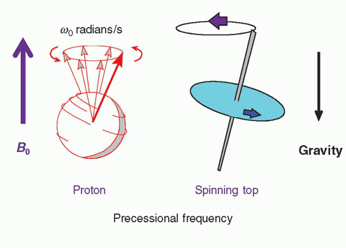
The magnetic moment of spins rotates around the static magnetic field, called precession, much in the same way that a spinning top wobbles due to the force of gravity (Fig. 12-4). The precession occurs at an angular frequency (number of rotations/s about an axis of rotation) that is proportional to the magnetic field strength B0. The Larmor equation describes the dependence between the magnetic field, B0, and the angular precessional frequency, ω0:


where γ is the gyromagnetic ratio unique to each nucleus. This is expressed in terms of linear frequency, where ω = 2πf and γ/2π is the gyromagnetic ratio, with values expressed in millions of cycles per second (MHz) per Tesla, or MHz/T.


Each nucleus with a non-zero nuclear magnetic moment has a unique gyromagnetic ratio, as listed in Table 12-2 (right column).


FIGURE 12-4 A single proton precesses about its axis at an angular frequency, ω, proportional to the externally applied magnetic field strength, according to the Larmor equation. A well-known example of precession is the motion a spinning top makes as it interacts with the force of gravity as it slows.


Typical magnetic field strengths for clinical MR systems range from 0.3 to 7.0 T. For protons, the precessional frequency is 42.58 MHz/T, and increases or decreases with an increase or decrease in magnetic field strength, as calculated in the example below. Accuracy of the precessional frequency is necessary to ensure that the RF energy will be absorbed by the magnetized protons. Precision of the precessional frequency must be on the order of cycles/s (Hz) out of millions of cycles/s (MHz) in order to identify the location and spatial position of the emerging signals, as is described in Section 12.6.

EXAMPLE: What is the frequency of precession of 1H and 31P at 0.5 T? 1.5 T? 3.0 T? The Larmor frequency is calculated as f0 = (γ/2π) B0.


FIELD STRENGTH


NUCLEUS


0.5 T


1.5 T


3.0 T


1H


42.58 × 0.5 = 21.29 MHz


42.58 × 1.5 = 63.87 MHz


42.58 × 3.0 = 127.74 MHz


31P


17.2 × 0.5 = 8.6 MHz


17.2 × 1.5 = 25.8 MHz


17.2 × 3 = 51.6 MHz


The differences in the gyromagnetic ratios and corresponding precessional frequencies allow the selective excitation of one element from another in the same magnetic field strength.


12.2 MR SYSTEM

The MR system is composed of several components including a magnet, magnetic field gradient coil, and radiofrequency (RF) coils, orchestrated by many processors and control subsystems, as shown in Figure 12-5. Details of the individual components, methods of acquiring the MR signals, and reconstruction of images are described in the following sections.


12.2.1 Magnets

The magnet is the heart of the MR system. For any magnet type, performance criteria include field strength, temporal stability, and field homogeneity. These parameters are affected by the magnet design. Air core magnets are made of wire-wrapped cylinders of approximately 1-m diameter and greater, over a cylindrical length of 2 to 3 m, where the magnetic field is produced by an electric current in the wires. When the wires are energized, the magnetic field produced is parallel to the long axis of the cylinder. In most clinically designed systems, the magnetic field is horizontal and runs along the cranial-caudal axis of the patient lying supine (Fig. 12-6A). Solid core magnets are constructed from permanent magnets, a wire-wrapped iron core “electromagnet,” or a hybrid combination. In these solid core designs, the magnetic field runs between the poles of the magnet, most often in a vertical direction (Fig. 12-6B). Magnetic fringe fields extend well beyond the volume of the cylinder in air core designs. Fringe fields are a potential hazard and are discussed further in Chapter 13.

To achieve a high magnetic field strength (greater than 1 T) requires the electromagnet core wires to be superconductive. Superconductivity is a characteristic of certain metals (e.g., niobium-titanium alloys) that when maintained at extremely low temperatures (liquid helium; less than 4 K) exhibit no resistance to electric current. Superconductivity allows the closed-circuit electromagnet to be energized and
ramped up to the desired current and magnetic field strength by an external electric source. Replenishment of the liquid helium must occur continuously, because if the temperature rises above a critical value, the loss of superconductivity will occur and resistance heating of the wires will boil the helium, resulting in a “quench.” Superconductive magnets with field strengths of 1.5 to 3 T are common for clinical systems.
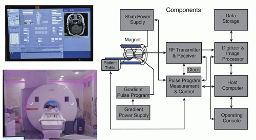


FIGURE 12-5 The MR system is shown (lower left), the operators display (upper left), and the various subsystems that generate, detect, and capture the MR signals used for imaging and spectroscopy.
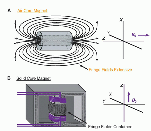


FIGURE 12-6 A. Air core magnets typically have a horizontal main field produced in the bore of the electrical windings, with the z-axis (B0) along the bore axis. Fringe fields for the air core systems are extensive and are increased for larger bore diameters and higher field strengths. B. The solid core magnet has a vertical field, produced between the metal poles of a permanent or wire-wrapped electromagnet. Fringe fields are confined with this design. In both types, the main field is parallel to the z-axis of the Cartesian coordinate system.


12.2.2 Magnetic Field Gradients

A magnetic field gradient is obtained by superimposing the magnetic fields of two or more coils carrying a direct current of specific amplitude and direction with a precisely defined geometry (Fig. 12-7). The bipolar gradient field varies over a predefined field of view (FOV), and when superimposed upon B0, a small, continuous variation in the field strength occurs from the center to the periphery with distance from the center point (the “null”). Interacting with the much, much stronger main magnetic field, the subtle linear variations are on the order of 0.004 T/m (4 mT/m) and are essential for localizing signals generated during the operation of the MR system.

Inside the magnet bore, three sets of gradients reside along the logical coordinate axes—x, y, and z—and produce a magnetic field variation determined by the magnitude of the applied current in each coil set (Fig. 12-8). When independently energized, the three coils (x, y, z) can produce a linearly variable magnetic field in any arbitrary direction, where the net gradient is equal to image
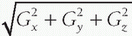
. Gradient polarity reversals (positive to negative and negative to positive changes in magnetic field strength) are achieved by reversing the current direction in the gradient coils. Two important properties of magnetic gradients are as follows: (1) The gradient field strength is determined by its peak amplitude and slope (change over distance), and typically ranges from 1 to 50 mT/m. (2) The slew rate is the time to achieve the peak magnetic field amplitude. Typical slew rates of gradient fields are from 5 to 250 mT/m/ms. As the gradient field is turned on, eddy currents are induced in nearby conductors such as adjacent RF coils and the patient, which produce magnetic fields that oppose the gradient field and limit the achievable slew rate. Actively shielded gradient coils and compensation circuits can reduce problems caused by eddy currents.
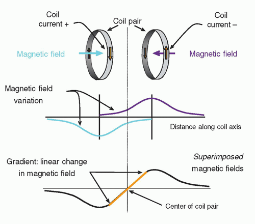
In a gradient magnetic field, protons maintain precessional frequencies corresponding to local magnetic field strength. At the middle of the gradient, called the gradient isocenter, there is no change in the field strength or precessional frequency. With a linear gradient, the magnetic field increases and decreases linearly in addition to the static magnetic field, as does the precessional frequency. The angular precessional frequency at a location within a linear gradient, ω, is


ω=γ(B0 + Gnet · d),

where Gnet is the net gradient and d is the distance from the gradient isocenter.


FIGURE 12-7 Gradients are produced inside the main magnet with coil pairs. Individual conducting wire coils are separately energized with currents of opposite direction to produce magnetic fields of opposite polarity. Magnetic field strength decreases with distance from the center of each coil. When combined, the magnetic field variations form a linear change between the coils, producing a linear magnetic field gradient, as shown in the lower graph.

EXAMPLE: What is the precession frequency of proton placed 20 cm from the gradient isocenter if the net gradient is 2 G/cm and the field strength is 1.5 T?

The B0 field strength is 1.5 T and the gradient adds a magnetic field of 40 G or 0.004 T (2 G/cm × 20 cm). The effective magnetic field strength at the location is 1.504 T. The Larmor frequency of proton at 1.504 T is 64.04 MHz (42.58 × 1.504). The Larmor frequency of proton increases by 0.17 MHz due to the gradient field.


FIGURE 12-8 Within the large stationary magnetic field, field gradients are produced by three separate coil pairs placed within the central core of the magnet, along the x, y, or z directions. In modern systems, the current loops are distributed across the cylinders for the x-, y-, and z-gradients, which generates a lower, but more uniform gradient field. Magnetic field gradients of arbitrary direction are produced by the vector addition of the individual gradients turned on simultaneously. Any gradient direction is possible by superimposition of magnetic fields generated by the three-axis gradient system.


12.2.3 Radiofrequency Coils

RF transmitter coils create an oscillating secondary magnetic field formed by passing an alternating current through a loop of wire. Irradiating the sample with an electromagnetic RF energy pulse tuned to the Larmor frequency induces the resonance of the magnetization within the sample. The magnetization along the direction of the static magnetic field, B0, shrinks with a simultaneous phase coherence that creates a perpendicular magnetization rotating at the Larmor frequency. This phenomenon is called excitation. To accomplish excitation and resonance, the created secondary field, called B1, must be arranged at right angles to the main magnetic field, B0. In an air core design with a horizontal field, the RF coil secondary field should be in the transverse or vertical axes, as the B1 field is created perpendicular to the transmit coils themselves. RF transmitter coils are therefore oriented above, below, or at the sides of the patient, and are usually cylindrical. In most systems, the body coil contained within the bore of the magnet is most frequently used, but also transmitter coils for the head, extremity, and some breast coils are coupled to a receiver coil.


The transverse magnetization within the sample returns to equilibrium conditions and releases detectable RF energy at the same frequency. While in phase coherence, the rotating magnetization vector generates a signal that is detected by highly sensitive antennas (RF receiver coils) to capture the basic MR signal. All RF receiver coils must resonate and efficiently store energy at the Larmor frequency. This is determined by the inductance and capacitance properties of the coil. RF transmit and receive coils need to be tuned prior to each acquisition and matched to accommodate the different magnetic inductance of each patient. Receiver coils must be properly placed to adequately detect the MR signal.

Very often, transmit and receive functions are separated to handle the variety of imaging situations that arise, and to maximize the SNR for an imaging sequence. Proximity RF coils include volume or bird-cage coils, the design of choice for brain imaging, the single-turn solenoid for imaging the extremities and the breasts, and the saddle coil. These coils are typically operated as both a transmitter and receiver of RF energy (Fig. 12-9A). Volume coils encompass the total area of the anatomy of interest and yield uniform excitation and SNR over the entire imaging volume. However, because of their relatively large size, images are produced with lower SNR than other types of coils. Enhanced performance is obtained with a process known as quadrature excitation and detection, which enables the energy to be transmitted and the signals to be received by two pairs of coils oriented at right angles, either electronically or physically. This detector manages two simultaneous channels known as the real (records MR information in phase with a reference signal) and the imaginary (records MR information 90° out of phase with the reference signal) channels, and increases
the SNR up to a factor of image. If imbalances in the offset or gain of these detectors occur, then artifacts will be manifested, such as a “center point” artifact.
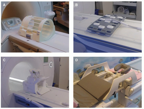


FIGURE 12-9 Radiofrequency surface coils improve image quality and SNR for specific examinations. A. A transmit/receive head coil. B. A flexible body coil and a spine coil imbedded on the table. C. A 64-channel phased array head and neck coil. D. A coil and a table dedicated for breast imaging and biopsy.

Phased array coils consisting of multiple coils and receivers are made of several overlapping loops, which extend the imaging FOV in one direction (Fig. 12-9B-D). The small FOV of each individual coil provides excellent SNR and resolution, and each is combined to produce a composite image with the advantages of the local surface coil, so that all data can be acquired in a single sequence. Phased array coils for the spine, pelvis, breast, cardiac, and temporomandibular joint applications are commonly purchased with an MR system for optimal image quality.

Surface coils are used to achieve high SNR and high resolution when imaging anatomy near the surface of the patient. They are typically receive-only designs and are usually small and shaped for a specific imaging exam and for patient comfort. The received signal sensitivity, however, is limited to the volume located around the coil at a depth into the patient equal to the radius of the coil, which causes a loss of signal with depth. There are now intracavitary coils for endorectal, endovascular, endovaginal, esophageal, and urethral local imaging, and they can be used to receive signals from deep within the patient. In general, a body coil is used to transmit the RF energy and the local coil is used to receive the MR signal.


12.2.4 MR System Subcomponents

The control interfaces, RF source, detector, and amplifier, analog to digital converter (digitizer), pulse programmer, computer system, gradient power supplies, and image display are crucial components of the MR system. They integrate and synchronize the tasks necessary to produce the MR image (Fig. 12-5).

The operator interface and computer systems vary with the manufacturer, but most consist of a computer system, dedicated processor for Fourier transformation, image processor to form the image, disk drives for storage of raw data and pulse sequence parameters, and a power distribution system to distribute and filter the direct and alternating current. The operator’s console is located outside of the scan room and provides the interface to the hardware and software for data acquisition (DAQ).

A cross section of the internal superconducting magnet components shows integral parts of the magnet system including the wire coils and cryogenic liquid containment vessel (Fig. 12-10). In addition to the main magnet system, other components are also necessary. Shim coils interact with the main magnetic field to improve homogeneity (minimal variation of the magnetic flux density) over the volume used for patient imaging. RF coils exist within the main bore of the magnet to transmit energy to the patient as well as to receive returning signals. Gradient coils are contained within the main bore to produce a linear variation of magnetic field strength across the useful magnet volume.


12.3 MAGNETIC RESONANCE SIGNAL

Application of RF energy synchronized to the precessional frequency of the protons causes absorption of energy and displacement of the sample magnetic moment from equilibrium conditions. The return to equilibrium results in the emission of energy proportional to the number of excited protons in the volume. This occurs at a rate that depends on the structural and magnetic characteristics of the sample. Excitation, detection, and acquisition of the signals constitute the basic information necessary for MRI and MRS.


FIGURE 12-10 Internal components of a superconducting air-core magnet are shown. On the left is a cross section through the long axis of the magnet illustrating relative locations of the components, and on the right is a simplified cross section across the diameter.
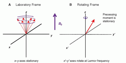

12.3.1 Orientation, Frame of Reference, and Magnetization Vectors

By convention, the applied magnetic field B0 is directed parallel to the z-axis of the three-dimensional Cartesian coordinate axis system and perpendicular to the x- and y-axes. For convenience, two frames of reference are used: the laboratory frame and the rotating frame. The laboratory frame (Fig. 12-11A) is a stationary reference frame from the observer’s point of view. The sample magnetic moment vector precesses about the z-axis in a circular geometry about the xy plane. The rotating frame (Fig. 12-11B) is a spinning axis system, whereby the x′-y′ axes rotate at an angular frequency equal to the Larmor frequency. In this frame, the sample magnetic moment vector appears to be stationary when rotating at the resonance frequency. A slightly higher precessional frequency is observed as a slow clockwise rotation, while a slightly lower precessional frequency is observed as a slow counterclockwise rotation. The magnetic interactions between precessional frequencies of the magnetic moments of the protons with the externally applied RF (depicted as a rotating magnetic field) can be described more clearly using the rotating frame of reference, while the observed returning signal and its frequency content is explained using the laboratory (stationary) frame of reference.

The net magnetization vector of the sample, M, is described by three components. Longitudinal magnetization, Mz, along the z direction, is the component of the magnetic moment parallel to the applied magnetic field, B0. At equilibrium, the longitudinal magnetization is maximal and is denoted as M0, the equilibrium magnetization. The component of the magnetic moment perpendicular to B0, Mxy, in the xy plane, is transverse magnetization. At equilibrium, Mxy is zero. When the protons in the magnetized sample absorb energy, phase coherence of the spins generates a rotating vector in the transverse plane, Mxy, generating the all-important MR signal. Figure 12-12 illustrates this geometry.


FIGURE 12-11 A. The laboratory frame of reference uses stationary three-dimensional Cartesian coordinates: x, y, z. The magnetic moment of the proton precesses around the z-axis at the Larmor frequency as the illustration attempts to convey. B. The rotating frame of reference uses rotating Cartesian coordinate axes that rotate about the z-axis at the Larmor precessional frequency, and the other axes are denoted: x′ and y′. When precessing at the Larmor frequency, the proton magnetic moment is stationary.


12.3.2 Resonance and Excitation

When a bar magnet continuously moves back and forth at the same (resonance) frequency of nearby magnetic spins pointing upward, the magnetic interaction causes the spins to tip downward to the perpendicular plane (Fig. 12-13A). Similarly, displacement of the equilibrium magnetization occurs when the magnetic component of the RF excitation pulse, known as the B1 field, is precisely matched to the precessional frequency of the protons (Fig. 12-13B). In the rotating frame, the B1 field continuously applies torque on the equilibrium magnetization when it is applied, causing displacement (Fig. 12-13C). If the B1 field is not applied at the precessional (Larmor) frequency, the B1 field will not interact with Mz (Fig 12-13D).


12.3.3 Flip Angles

Flip angles represent the degree of Mz rotation by the B1 field as it is applied along the x′-axis (or the y′-axis) perpendicular to Mz. A torque is applied on Mz, rotating it from the longitudinal direction into the transverse plane. The rate of rotation
occurs at an angular frequency equal to ω1 = γB1 as per the Larmor equation. Thus, for an RF pulse (B1 field) applied over a time t, the magnetization vector displacement angle, θ, is determined as θ = ω1t = γB1t, and the product of the pulse time and B1 amplitude determines the displacement of Mz. This is illustrated in Figure 12-14.
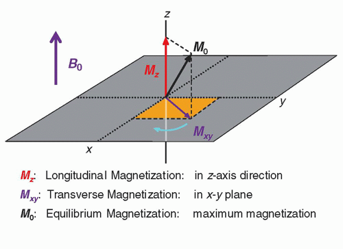


FIGURE 12-12 Longitudinal magnetization, Mz, is the vector component of the magnetic moment in the z direction. Transverse magnetization, Mxy, is the vector component of the magnetic moment in the x-y plane. Equilibrium magnetization, M0, is the maximum longitudinal magnetization of the sample, and is shown displaced from the z-axis in this illustration.
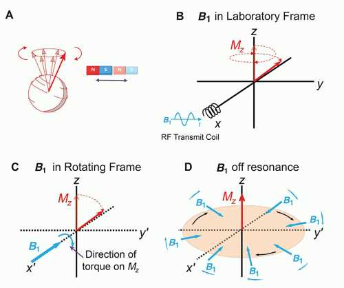


FIGURE 12-13 An intuitive description of magnetic resonance. A. A small magnet near a magnetic dipole moving back and forth at the resonance frequency increases the energy in the dipole and induces larger oscillation, an “excited” state. B. In the laboratory frame, sinusoidal magnetic fields generated by a coil in the x-axis excites the magnetic moment in the z-axis into the xy plane. C. In the rotating frame, the RF pulse (B1 field) is applied at the Larmor frequency and is stationary in the x′-y′ plane. The B1 field interacts at 90° to the sample magnetic moment and produces a torque that displaces the magnetic vector away from equilibrium. D. The B1 field is not tuned to the Larmor frequency and is not stationary in the rotating frame. No interaction with the sample magnetic moment occurs.
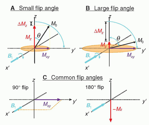
Common flip angles are 90° (π/2) and 180° (π), although a variety of smaller and larger angles are chosen to enhance tissue contrast in various ways. A 90° angle provides the largest possible Mxy and detectable MR signal and requires a known B1 strength and time (on the order of a few to hundreds of µs). The displacement angle of the sample magnetic moment is linearly related to the product of B1 field strength and time: For a fixed B1 field strength, a 90° displacement takes half the time of a 180° displacement. With flip angles smaller than 90°, less time is needed to displace Mz, and a larger transverse magnetization per unit excitation time is achieved. For instance, a 45° flip takes half the time of a 90° flip yet creates 70% of the signal, as the magnitude of Mxy is equal to the sine of 45°, or 0.707. With fast MRI techniques, small displacement angles of 10° and less are often used.


FIGURE 12-14 Flip angles describe the angular displacement of the longitudinal magnetization vector from the equilibrium position. The rotation angle of the magnetic moment vector is dependent on the duration and amplitude of the B1 field at the Larmor frequency. Flip angles describe the rotation of Mz away from the z-axis. Small flip angles (less than 45°) (A) and large flip angles (75° to 90°) (B) produce small and large transverse magnetization, respectively. C. Common flip angles are 90°, which produce the maximum transverse magnetization, and 180°, which invert the existing longitudinal magnetization to –Mz.
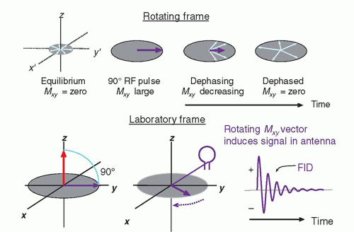

12.4 MAGNETIZATION PROPERTIES OF TISSUES


12.4.1 Free Induction Decay: T2 and T2* Relaxation

After a 90° RF pulse is applied to a magnetized sample at the Larmor frequency, an initial phase coherence of the individual protons is established and maximum Mxy is achieved. Rotating at the Larmor frequency, the transverse magnetic field of the excited sample induces signal in the receiver antenna coil (in the laboratory frame of reference). A damped sinusoidal electronic signal, known as the free induction decay (FID), is produced (Fig. 12-15).


FIGURE 12-15 Top: Conversion of longitudinal magnetization, Mz, into transverse magnetization, Mxy, results in an initial phase coherence of the individual spins of the sample. The magnetic moment vector precesses at the Larmor frequency (stationary in the rotating frame), and dephases with time. Bottom: In the laboratory frame, Mxy precesses and induces a signal in an antenna receiver sensitive to transverse magnetization. An FID signal is produced with positive and negative variations oscillating at the Larmor frequency, and decaying with time due to the loss of phase coherence.


The FID amplitude decay is caused by loss of Mxy phase coherence due to intrinsic micromagnetic inhomogeneities in the sample’s structure, whereby individual protons in the bulk water and hydration layer coupled to macromolecules precess at incrementally different frequencies arising from the slight changes in local magnetic field strength. Phase coherence is lost over time as an exponential decay. Elapsed time between the peak transverse signal (e.g., directly after a 90° RF pulse) and 37% of the peak level (1/e) is the T2 relaxation time (Fig. 12-16A). Mathematically, this is expressed as


where Mxy(t) is the transverse magnetic moment at time t for a sample that has M0 transverse magnetization at t = 0. When t = T2, then e-1 = 0.37 and Mxy = 0.37 M0. The molecular structure of the magnetized sample and characteristics of the bound water protons strongly affects its T2 decay value. Amorphous structures (e.g., cerebral spinal fluid [CSF] or highly edematous tissues) contain mobile molecules with fast and rapid molecular motion. Without structural constraint (e.g., lack of a hydration layer), these tissues do not support intrinsic magnetic field inhomogeneities, and thus exhibit long T2 values. As molecular size increases for specific tissues, constrained molecular motion and the presence of the hydration layer produce magnetic field domains within the structure and increase spin dephasing that causes more rapid decay with the result of shorter T2 values. For large, non-moving structures, stationary magnetic inhomogeneities in the hydration layer result in these types of tissues (e.g., bone) having a very short T2.

Extrinsic magnetic inhomogeneities, such as the imperfect main magnetic field, B0, or susceptibility agents in the tissues (e.g., MR contrast materials, paramagnetic or ferromagnetic objects), add to the loss of phase coherence from intrinsic inhomogeneities and further reduce the decay constant, known as T2* under these conditions (Fig. 12-16B).

Only gold members can continue reading. Log In or Register to continue

Stay updated, free articles. Join our Telegram channel

May 16, 2021 | Posted by in GENERAL RADIOLOGY | Comments Off on Magnetic Resonance Basics: Magnetic Fields, Nuclear Magnetic Characteristics, Tissue Contrast, Image Acquisition

Full access? Get Clinical Tree

Get Clinical Tree app for offline access