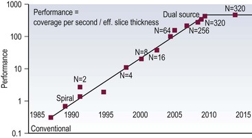
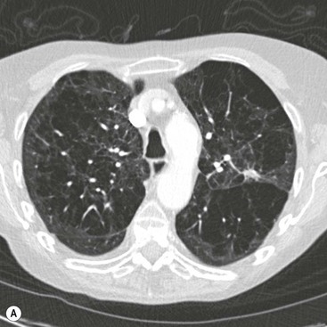
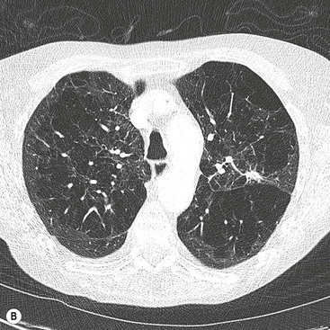
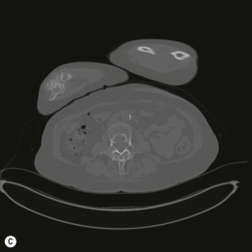
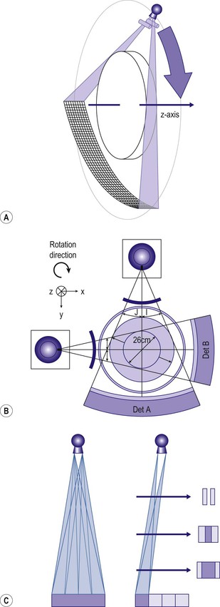
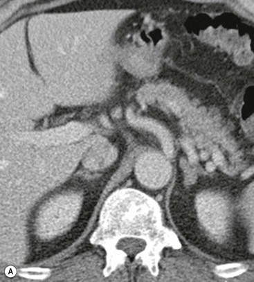
Ashley S. Shaw, Mathias Prokop In 1917, Johann Radon, an Austrian mathematician, presented an algorithm for creating an image from a set of measured projection data. However, it took almost 50 years before theoretical physics and mathematics were developed far enough to allow construction of such a device By the early 1970s, further significant advances in computing and increased understanding of the mathematics of line integrals and Fourier analysis enabled a prototype CT machine to be developed.1,2 The first CT machine used for clinical purposes, developed by the late Sir Godfrey Hounsfield, was installed at the Atkinson Morley Hospital, London, in the early 1970s. Each axial image of the head took several minutes to acquire and days to reconstruct at the laboratories of the record company EMI. Over the next decade, CT machines became faster as the processing power of computers improved. Intravenous contrast material injection was used to better delineate abnormalities. Still, the body had to be examined one slice at a time, which made total acquisition slow and hampered the exploitation of the differential contrast enhancement occurring in the various phases after contrast injection. The only way to exploit this was dynamic image acquisition at one predefined anatomical level. Techniques such as CT perfusion and dual energy were introduced at that time. In the late 1980s, the development of slip-ring technology enabled continuous revolution of the X-ray unit, which not only reduced the acquisition time per axial image to 1 s but also allowed helical data to be acquired.3 This revolutionised CT because whole organ systems could now be examined continuously during a single breath hold. This removed problems of reproducibility of breath hold levels and allowed for CT data acquisition during predefined phases of enhancement with intravenous contrast agents. CT data acquisition in the arterial phase and CT angiography could be introduced. Computer analysis of routine helical CT acquisitions provided 3D data sets allowing multiplanar reconstructions, but the spatial resolution was still substantially higher in the original axial images than in the coronal or sagittal reformatted images. The next step of development occurred in the late 1990s, when detectors were split into multiple thin rows along the z-axis to permit acquisition of multiple sections simultaneously (multidetector CT). This decreased acquisition time yet further and made it possible to routinely use thin sections. As a result, multidetector CT is nowadays able to provide near isotropic volumetric data sets in which spatial resolution is similar in all planes. The 2000s saw the introduction of cardiac CT which is based on ECG-synchronisation to freeze cardiac motion. The number of detector rows increased from 4 to somewhere between 64 and 320 rows, depending on the manufacturer. Rapid tube rotation (<0.3 s) and dual-source systems with two X-ray tubes were developed to optimise cardiac imaging. The exponential doubling of CT performance every two years4 in the 1980s, 1990s and 2000s slowed around 2010 (Fig. 4-1). CT presents itself nowadays as a mature technology. Current developments focus on reducing radiation exposure and further exploitation of dual-energy CT, dynamic imaging and CT perfusion techniques. CT involves the imaging of thin axial sections of the body with X-rays. The X-rays pass through the body and are detected by a detector positioned on the opposite side of the body. The projection data must be acquired from multiple angles around the body. From these raw data, a computer reconstructs a map of the local attenuation within the examined section. Each image in the transverse (= axial) plane consists of a matrix of data points (picture elements, pixels) that are assigned a number that represents the X-ray attenuation (µ) at that particular point in the body. This CT number is actually a scaled version of µ that is normalised to the X-ray attenuation of water µW: CT = 1000 × (µ/µW − 1). The resulting numbers are called ‘Hounsfield units’ (HU). As a result of the normalisation, air is assigned a CT number of −1000 HU and water is assigned 0 HU. The CT numbers of solid soft tissues are centred around 0 HU, the lungs around −1000 HU and bone usually well above 200 HU, with dense cortical bone often nearing +1000 HU. The size of the image matrix used in modern multidetector CT systems is usually 512 × 512 pixels. However, some manufacturers provide 768 and 1024 matrices for high-resolution applications. The pixel size is derived from the reconstructed field of view (FOV) and the matrix size. For body applications, the pixel size is usually in the range of 0.6–0.8 mm, for the brain it is approximately 0.5 mm and for extremities it varies between 0.3 and 0.5 mm. Each pixel collects attenuation data from a corresponding small volume (voxel) within the body region being examined by CT. The body is represented in a CT data set as a 3D matrix. Each matrix element contains the CT number of its respective voxel in the human body although voxels within a CT matrix usually overlap. This is most apparent when data sets are reconstructed with a reconstruction interval that is smaller than the section thickness used for the original image acquisition. The first- and second-generation CT machines constructed in the 1970s and early 1980s were limited by complex motion patterns that made it time-consuming to acquire a single image. Third-generation CT systems had an X-ray tube rotate around the patient. Fourth-generation CT machines employed a static ring of detectors with a rotating tube. The physical hard-wiring of the tube, however, allowed for only one revolution at a time before having to ‘unwind’ the tube. Slip-ring technology introduced in the late 1980s enabled continuous rotation of the X-ray tube (and detectors) synchronously around the patient. Helical (or spiral CT) is based on a continuously rotating tube and simultaneous movement of the patient through the image acquisition fan plane. Instead of the original stop and start acquisitions, helical CT provided true volumetric acquisitions. Multidetector CT technology then split the detector into multiple thin rows (Fig. 4-2A), thus allowing simultaneous acquisition of multiple axial sections to be obtained during one rotation of the tube. All multidetector systems use third-generation technology with rotating tube and detectors because of better scatter suppression and lower detector cost compared with a fourth-generation setup. Indeed the whole original concept of ‘generations’ has been somewhat superseded by the further development of tubes, detectors and reconstruction processes. Most current CT machines employ a single X-ray tube and require at least a 180° rotation to supply sufficient data for image reconstruction. Dual-source CT machines, however, employ two separate tube/detector systems lying roughly perpendicular to each other (Fig. 4-2B) and require only a 90° rotation to supply the 180° of projectional data required for image reconstruction. Tube designs have improved substantially over the past decades and nowadays are able to deliver sufficient radiation even during the very short acquisition times of 80–200 ms required for cardiac CT. Usually, X-ray tubes use a fixed focal spot to create radiation. Flying focal spot techniques vary the position of the X-ray focus on the tube anode so that slightly different projections are created during one tube rotation around the patient (Fig. 4-2C). This technique reduces aliasing effects and improves image quality. The focus originally was switched between two points parallel to the acquired CT section (xy-plane). Many modern CT systems now also allow acquisition of added projections in the z-direction (z-flying focal spot, z-FFS). Since it doubles the number of projections in the z-direction, the technique has been used as an argument to refer to CT systems with 32 rows of detectors as ‘64-slice’ machines. However, while a z-FFS does reduce aliasing artefacts in the z-direction, it does not double maximum coverage, maximum speed or maximum resolution, all factors that characterise a true 64-detector CT system. The detectors used in CT typically comprise several components: a scintillator absorbs the X-rays and converts them into visible light. The light in turn stimulates a photodiode to produce an electrical signal from which the image can be constructed. In order to improve spatial resolution, detectors have become smaller (typically around 0.5 mm in the direction of the acquisition plane and 1 mm in the z-direction), more sensitive (allowing some dose reduction) and react faster (allowing increased gantry rotation speeds). Better construction of modern detectors also reduces the length of wiring and, thus, electrical noise, a factor that is essential for low-dose imaging. Detectors used for multidetector CT consist of multiple parallel rows of detector elements. Due to the cone shape of the X-ray beam and the usual enlargement of an object at the centre of the field of view (e.g. the human torso), the width of the detector rows is roughly double that of the minimum section thickness available. Most current CT systems do not vary the width of these detector rows but some use wider detector rows towards the edge of the detector array. CT systems are now usually classified by the maximum number of rows of detectors that can be used simultaneously (4-row, 16-row, 64-row, 320-row systems, etc.). In most systems, the terms ‘row’ and ‘slice’ can be used interchangeably, which means that a 64-slice multidetector CT system usually has 64 rows of detectors. The exception are systems with a z-FFS (see above), in which a 64-slice CT system, for example, signifies actually has only 32 rows but they are doubled due to an oscillating focal spot. The confusion is further increased by the fact that in the first years of multidetector CT the number of axial slices that could be reconstructed from one rotation was equal to the number of slices indicated in the name of the CT system; for example, exactly 16 axial slices could be reconstructed from one rotation of a multidetector composed of 16 units. However, on a 64-slice CT system with a z-FFS the maximum number of slices that could be reconstructed from one rotation was only 32. As reconstruction technology evolved and detectors became even wider, sections could be reconstructed in an overlapping fashion from data acquired during one rotation. This made it possible to reconstruct, for example, 640 axial slices from one rotation of a 320-slice CT system. The consequence of the ‘slice wars’ of the late 2000s, in which vendors tried to outdo each other with the performance parameters of their CT systems, is that the user must be careful to fully understand what stands behind each technology. Thus, 16-row multidetector CT systems were able to acquire data with submillimetre resolution in all planes in 10 s or less for most organ systems. A 64-slice CT system was able to do the same, but even faster, and added good cardiac capabilities. While vendors chose relatively parallel technological paths in the past, their more recent development paths are diverging. Dual-source technology focuses on speed for cardiac imaging. Wide detectors aim to cover large areas of anatomy, ideally a whole organ such as heart or liver, within one rotation. They reduce artefacts between adjacent sections and are well suited for perfusion imaging. Faster rotation speed has been developed to reduce (cardiac) motion artefacts. Dual-energy imaging is achieved using dual-source technology, rapid kV switching, dual rotation techniques and sandwich detectors for separating high- and low-energy photons. Some techniques, like ultrafast ‘flash’ or single-shot CT, are limited to CT systems from particular vendors. In general, however, most clinical questions can very well be answered with current 64-slice technology. When it comes to high-end applications, each user must carefully weigh up the clinical requirements for advanced imaging and the capabilities of each technology platform. In order to be able to calculate a CT image (axial image data) from projectional raw CT data acquired from various angles, the section must be sampled adequately. For third-generation geometry, data from at least a 180° rotation are required. CT data acquisitions that involve 180° of data are called ‘half-scan’ reconstructions, while those that involve a full 360° rotation are called ‘full-scan’ reconstructions. Because of a better image quality, full 360° rotation acquisitions are standard in clinical practice, but 180° rotation acquisitions can be superior because of a shorter sampling duration whenever motion is to be suppressed, particularly during cardiac imaging. The reconstruction process involves a technique called filtered back projection (FBP) in which the raw data is first filtered and then projected back over the area that needs to be reconstructed. The result is a CT image in which the spatial resolution is determined by the sharpness of the filter kernel used for reconstruction (Fig. 4-3). With the increasing width of modern detectors, the slice geometry can no longer be approximated by a thin parallel beam but must consider the fact that the X-ray beam diverges also in the z-direction. Various techniques to compensate for this effect have been developed. Adaptive multiplanar reconstruction (AMPR), for example, reconstructs intermediate data consisting of a vast number of half-scans in planes that best fit the fan-beam trajectory and wobble around the z-axis. Images in arbitrary planes can be reconstructed from the raw data by interpolating the intermediate data. AMPR works well for modest cone angles. As cone angles get wider, so-called Feldkamp algorithms that mathematically correct for the cone geometry must be used but these are computationally expensive and relatively time-consuming. Nevertheless, cone beam CT is gaining certain applications where rapid imaging is required—vascular and interventional are examples. With increasing power of modern computers, image reconstruction can also be performed using an iterative optimisation step. Ideally, the projection data derived from the calculated image are compared with the original data. Reconstruction is stopped as soon as these two entities are reasonably similar. This so-called ‘iterative reconstruction’ (IR) is much more time-consuming than FBP but is also much less affected by random variations (quantum or electronic noise) in the raw data. The result is either superior image quality or lower radiation dose requirements for IR. In practice, IR is now often used to provide similar image quality but with a lower radiation dose and, sometimes, a lower dose of intravenous contrast agent.5 Most vendors nowadays offer iterative reconstruction as a routine but the chosen techniques vary substantially. Some only involve image data and act like an advanced noise-reducing filter. Techniques that only use raw data can integrate realistic information about detector geometry, electronic noise, quantum statistics, tube filtering, etc., to create excellent image quality at massively reduced radiation dose and with fewer artefacts. The penalty, however, is the extremely long reconstruction, even with dedicated hardware. For this reason, most techniques use image data as well as raw data to achieve a good compromise between reconstruction speed, image quality and noise reduction. One must be aware, however, that even IR cannot retrieve information that is not there: at very low-dose levels, low-contrast resolution suffers first, and the image can have a ‘plasticy’ look that will reduce acceptance among radiologists (Fig. 4-4).
Computed Tomography
Computed Tomography (CT): A Brief History
Principles of Computed Tomography
CT Numbers and Image Matrix
Generations of CT Development
X-Ray Tubes
X-Ray Detectors
Slice Wars and Beyond
Image Reconstruction
Filtered Back Projection
Iterative Reconstruction
Related posts:
![]()
Stay updated, free articles. Join our Telegram channel

Full access? Get Clinical Tree