COMPUTED TOMOGRAPHY

OUTLINE

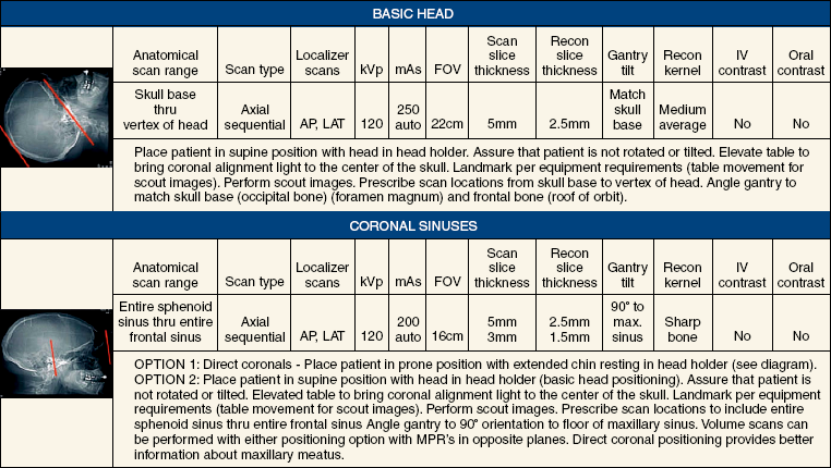
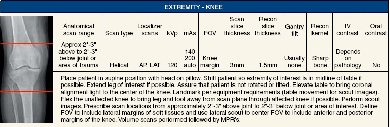
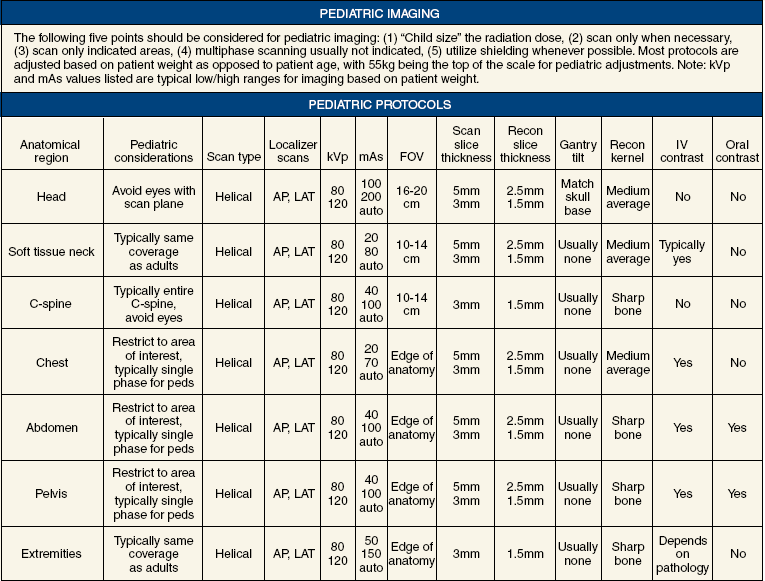
Basic Computed Tomography Examination Protocols

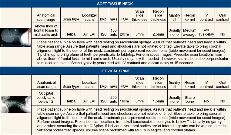
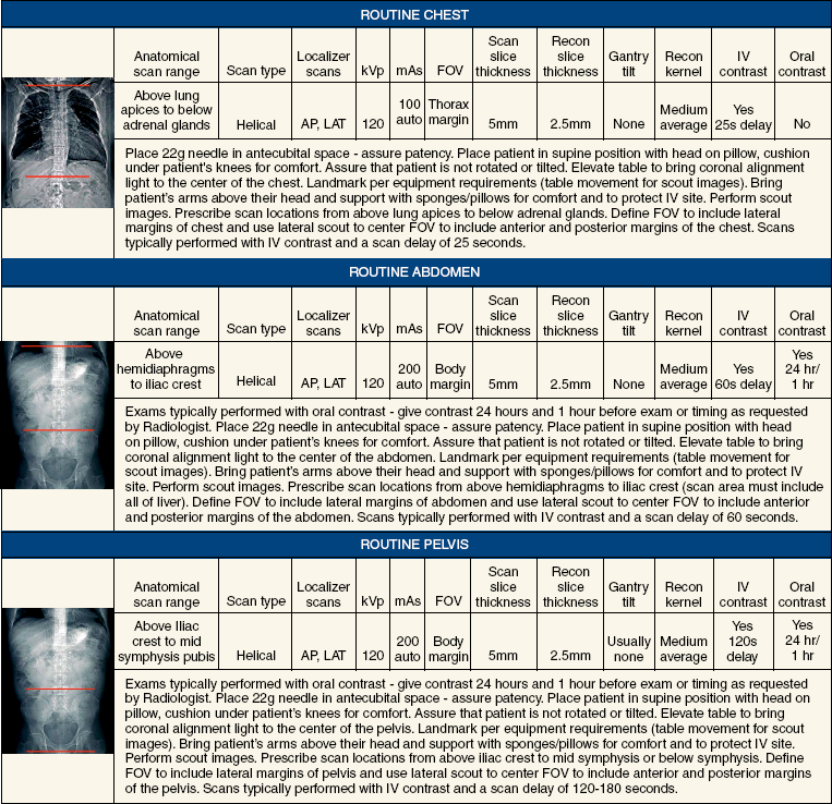
Because of the numerous scanner types, parameters, tube rotation speeds, and detector types that are used in computed tomography (CT) imaging, it is impossible to list exact examination protocols. Technical factors are directly related to the detector configuration that is used: number of detector rows and fixed array versus adaptive array. Many scans are performed using auto tube current modulation as opposed to fixed mA. This chapter is an overview of basic CT scan protocols using an adaptive array, 16-row scanner. The values listed are close approximations of what can be used for the various examinations.

Fundamentals of Computed Tomography

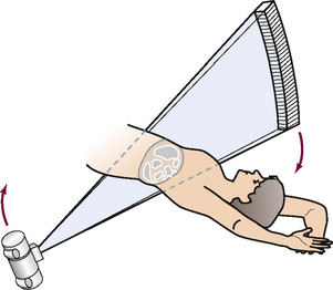
Computed tomography (CT)^* is the process of creating a cross-sectional tomographic plane of any part of the body (Fig. 31-1 ). For CT, a patient is scanned by an x-ray tube rotating around the body part being examined. A detector assembly measures the radiation exiting the patient and feeds back the information, referred to as primary data, to the host computer. After the computer has compiled and calculated the data according to a preselected algorithm, it assembles the data in a matrix to form an axial image. Each image, or slice, is displayed in a cross-sectional format.

Fig. 31-1 CT scanner provides cross-sectional images by rotating around the patient.

In the early 1970s, CT scanning was used clinically only for imaging of the brain. The first CT scanners were capable of producing only axial images and were called CAT (computed axial tomography) units by the public; this term is no longer accurate because images can now be created in multiple planes. In the past few decades, dramatic technical advancements have led to the development of CT scanners that can be used to image virtually every structure within the human body. Improvements in scanner design and computer science have produced CT units with new imaging capabilities and reconstruction techniques. Three-dimensional reconstructions of images of the internal structures are used for surgical planning, CT angiography (CTA), radiation therapy planning, and virtual reality imaging.

CT-guided biopsies and fluid drainage offer an alternative to surgery for some patients. Although these procedures are considered invasive, they offer shorter recovery periods, no exposure to anesthesia, and less risk of infection. CT is also used in radiation oncology for radiation therapy planning. CT scans taken through the treatment field, with the patient in treatment position, have drastically improved the accuracy and quality of radiation therapy.

Computed Tomography and Conventional Radiography

When a conventional x-ray exposure is made, the radiation passes through the patient and produces an image of the body part. Frequently, body structures are superimposed (Fig. 31-2 ). Visualizing specific structures requires the use of contrast media, varied positions, and usually more than one exposure. Localization of masses or foreign bodies requires at least two exposures and a ruler calibrated for magnification.

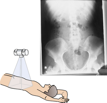
Fig. 31-2 Conventional radiograph superimposes anatomy and yields one diagnostic image with fixed density and contrast.

During the CT examination, a tightly collimated x-ray beam is directed through the patient from many different angles, resulting in an image that represents a cross section of the area scanned. This imaging technique essentially eliminates the superimposition of body structures. The CT technologist controls the method of acquisition, the slice thickness, the reconstruction algorithm, and other factors related to image quality.

In the digital radiograph of the abdomen shown in Fig. 31-3 , high-density bone and low-density gas are seen, but many soft tissue structures, such as the kidneys and intestines, are not clearly identified. Contrast media are needed to visualize these structures. A CT examination of the abdomen would show all of the structures that lie within the slice. In Fig. 31-4, A , the liver, stomach, kidneys, spleen, and aorta can be identified. In addition to eliminating superimposition, CT is capable of differentiating among tissues with similar densities. This differentiation of densities is referred to as contrast resolution. The improved contrast resolution with CT compared with conventional radiography is due to a reduction in the amount of scattered radiation.

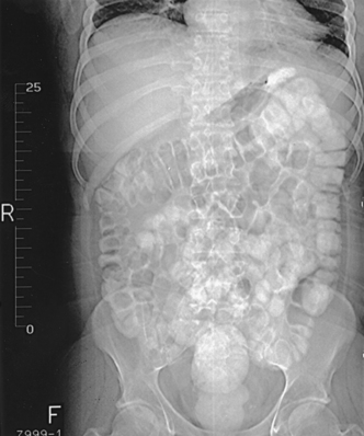
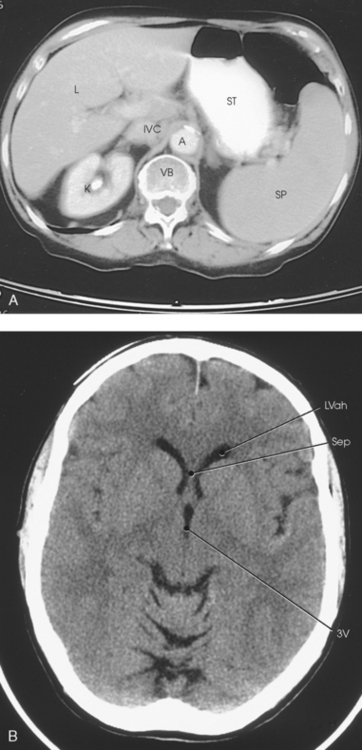
Fig. 31-3 Digital kidney, ureter, and bladder (KUB).

Fig. 31-4 A, Axial image of abdomen showing liver (L), stomach (ST), spleen (SP), aorta (A), inferior vena cava (IVC), vertebral body of thoracic spine (VB), and kidney (K). B, Axial CT scan of lateral ventricles (LVah), septum (Sep), and third ventricle (3V). (B, From Kelley LL, Petersen CM: Sectional anatomy for imaging professionals, ed 2, St Louis, 2007, Mosby.)

Fig. 31-4, B, is an axial image of the brain that differentiates the gray matter from the white matter and shows bony structures and cerebrospinal fluid within the ventricles. Because CT can show subtle differences in various tissues, radiologists are able to diagnose pathologic conditions more accurately than if they were to rely on radiographs alone. Because the image is digitized by the computer, numerous image manipulation techniques can be used to enhance and optimize the diagnostic information available to the physician (Fig. 31-5 ).

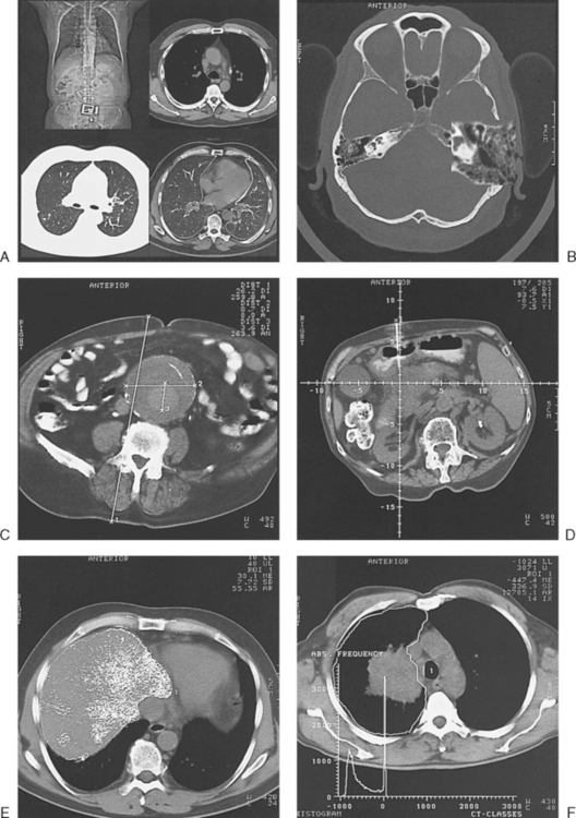
Fig. 31-5 Image manipulation techniques used to enhance diagnostic information in CT image. A, Multiple imaging and windows. B, Image magnification. C, Measurement of distances. D, Superimposition of coordinates on the image. E, Highlighting. F, Histogram. (Courtesy Siemens Medical Systems, Iselin, NJ.)

Historical Development

CT was first performed successfully in 1970 in England at the Central Research Laboratory of EMI, Ltd. Hounsfield, an engineer for EMI, and Cormack, a nuclear physicist from Johannesburg, South Africa, are generally given credit for the development of CT. For their research, they were awarded the Nobel Prize in Medicine and Physiology in 1979. After CT was shown to be a useful clinical imaging modality, the first full-scale commercial unit, referred to as a brain tissue scanner, was installed in Atkinson Morley’s Hospital in 1971. An early dedicated head CT scanner is shown in Fig. 31-6 . Physicians recognized its value for providing diagnostic neurologic information, and its use was accepted rapidly. The first CT scanners in the United States were installed in June 1973 at the Mayo Clinic, Rochester, Minnesota, and later that year at Massachusetts General Hospital, Boston. These early units were also dedicated head CT scanners. In 1974, Ledley at Georgetown University Medical Center, Washington, D.C., developed the first whole-body scanner, which greatly expanded the diagnostic capabilities of CT.

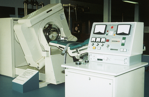
Fig. 31-6 First-generation EMI CT unit: dedicated head scanner. (Photograph taken at Reöntgen Museum, Lennep, Germany.)

After CT was accepted by physicians as a diagnostic modality, numerous companies in addition to EMI began manufacturing scanners. Although the units differed in design, the basic principles of operation were the same.

Computed Tomography Scanner Generation Classifications

CT scanners have been categorized by generation, which is a reference to the level of technologic advancement of the tube and detector assembly. The original “generation” classification of scanners was a clear distinction of tube movement versus detector rotational path. As scanner technology has progressed, the tube movement and detector rotation relationship has remained relatively constant, but the tube power source and the detector configurations have changed. Some authors have used slip ring or detector advancements to assign a generation number. These varied opinions and discussions have led to some confusion concerning scanner generation classifications. The following discussion of scanner generations follows the original standards of tube movement versus detector rotation.

The early units, referred to as first-generation scanners, worked by a process known as translate/rotate. The tube produced a finely collimated beam, or pencil beam. Depending on the manufacturer, one to three detectors were placed opposite the tube for radiation detection. The linear tube movement (translation) was followed by a rotation of 1 degree. Scan time was usually 3 to 5 minutes per scan, which required the patient to hold still for extended periods. Because of the slow scanning and reconstruction time, the use of CT was limited almost exclusively to neurologic examinations. A CT image from a first-generation scanner is shown in Fig. 31-7 .

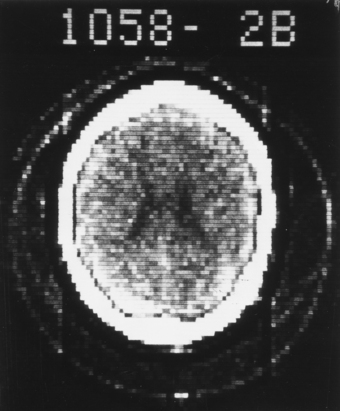
Fig. 31-7 Axial brain image from the first CT scanner in operation in the United States: Mayo Clinic, Rochester, Minnesota. The 80 × 80 matrix produced a noisy image. The examination was performed in July 1973.

The second-generation scanners were considered a significant improvement over first-generation scanners. The x-ray tube emitted a fan-shaped beam that was measured by approximately 30 detectors placed closely together in a detector array. Tube and detector movement was still translate/rotate; however, the gantry rotated 10 degrees between each translation. These changes improved overall image quality and decreased scan time to about 20 seconds for a single slice. The time required to complete one CT examination remained relatively long, however.

The third–generation scanners introduced a rotate/rotate movement, in which the x-ray tube and detector array rotate simultaneously around the patient. An increase in the number of detectors (>750) and their arrangement in a “curved” detector array considerably improved image quality (Fig. 31-8 ). Scan times were decreased to 0.35 to 10 seconds per slice, which made the CT examination much easier for patients and helped decrease motion artifact. Advancements in computer technology also decreased image reconstruction time, substantially reducing examination time. Most current scanners are third-generation configurations with one of the following technical variations:

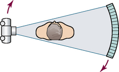
Fig. 31-8 Rotate/rotate movement: tube and detector movement of a thirdgeneration scanner.

• Helical CT, single-slice helical CT (SSHCT). Slip-ring technology allows 360-degree continuous rotation of tube and detector. Reduces scan times to subsecond per slice.

• Multislice detectors (MSHCT or MDCT). Increase in number of detector rows allows multiple slices to be taken in one rotation. As detector rows increase, the fan beam geometry of the x-ray beam has been adapted. Began with two-slice scanners and quickly moved to four-slice and more.

• Volume CT (VCT). Multislice scanners with 64 detector rows or more. The x-ray beam geometry must be a cone-beam configuration to accommodate the increased length of the scanner.

• Flat-panel CT (FP-CT or FD-CT). A detector plate similar to plates used in digital radiography (DR) replaces the typical detector configuration. In dedicated breast units, the tube and detector travel a full 360 degrees. In other applications, the unit functions more like a C-arm fluoroscopy unit in which the tube and detector do not travel in a full 360 degrees. Scanners provide excellent spatial resolution but lower contrast resolution.

The fourth-generation scanners introduced the rotate-only movement in which the tube rotates around the patient, but the detectors were in fixed positions, forming a complete circle within the gantry (Fig. 31-9 ). The use of stationary detectors required greater numbers of detectors to be installed in a scanner. Fourth-generation scanners tended to yield a higher patient dose per scan than previous generations of CT scanners.

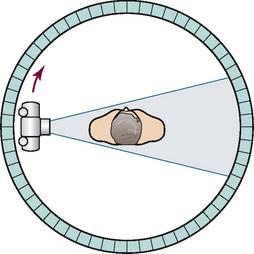
Fig. 31-9 Rotate-only movement: tube movement with stationary detectors of a fourth-generation scanner.

The fifth-generation scanners are classified as high-speed CT scanners because of millisecond acquisition times. These scanners are electron-beam scanners (EBCT) in which x-rays are produced from an electron beam in a fan beam configuration that strikes stationary tungsten target rings (Fig. 31-10 ). The detector rings are in a ±210-degree arc. These scanners were primarily used for cardiac studies.

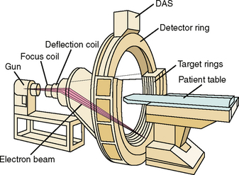
Fig. 31-10 Electron beam CT scanner configuration. X-rays, produced from electron beam, strike four target rings.

The sixth-generation scanners are dual-energy source (two x-ray tubes) (DSCT, DE-CT) that have two sets of detectors that are offset by 90 degrees. These DSCT scanners provide improved temporal resolution needed for imaging moving structures such as the heart (Fig. 31-11 ). The original DSCT scanners had several technical challenges and were not widely used. The latest DSCT scanners have solved the technical issues, however, and offer dual-energy capabilities between the two CT tubes. This technology allows a marked decrease in patient radiation dose.

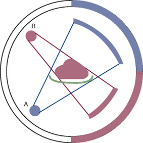
Fig. 31-11 Dual-source CT scanner (DSCT) configuration. This is considered a sixth-generation scanner.

Most scanners in use today are a third-generation variation that have 4 to 320 rows of detectors in a single array. This increase in numbers of detector rows has increased the length of the detector, which requires the x-ray beam to be cone-shaped to encompass the full detector array. This is a change from the original third-generation fan beam. The flat panel detector also requires cone-beam geometry. The increased detector size and the cone-beam geometry pose various challenges in maintaining image quality, but this is a discussion that is too involved for this chapter.

Technical Aspects

The axial images acquired by CT scanning provide information about the positional relationships and tissue characteristics of structures within the section of interest. The computer performs a series of steps to generate one axial image. With the patient and gantry perpendicular to each other, the tube rotates around the patient, irradiating the area of interest. For every position of the x-ray tube, the detectors measure the transmitted x-ray values, convert them into an electrical signal, and relay the signal to the computer. The measured x-ray transmission values are called projections (scan profiles) or raw data. When collected, the electrical signals are digitized, a process that assigns a whole number to each signal. The value of each number is directly proportional to the strength of the signal.

The digital image is an array of numbers arranged in a grid of rows and columns called a matrix. A single square, or picture element, within the matrix is called a pixel. The slice thickness gives the pixel an added dimension called the volume element, or voxel. Each pixel in the image corresponds to the volume of tissue in the body section being imaged. The voxel volume is a product of the pixel area and slice thickness (Fig. 31-12 ). The field of view (FOV) determines the amount of data to be displayed on the monitor.

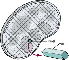
Fig. 31-12 CT image is composed of a matrix of pixels, with each pixel representing a volume of tissue (voxel).

Each pixel within the matrix is assigned a number that is related to the linear attenuation coefficient of the tissue within each voxel. These numbers are called CT numbers or Hounsfield units. CT numbers are defined as a relative comparison of x-ray attenuation of a voxel of tissue with an equal volume of water. Water is used as reference material because it is abundant in the body and has a uniform density; water is assigned an arbitrary value of 0. Tissues that are denser than water are given positive CT numbers, and tissues with less density than water are assigned negative CT numbers. The scale of CT numbers ranges from −1000 (air/gas) to +3000 (dense bone). Average CT numbers for various tissues are listed in Table 31-1 .

TABLE 31-1

Average Hounsfield units (HU) for selected substances

Substance	HU
Air	−1000
Lungs	−250 to −850
Fat	−100
Orbit	−25
Water	0
Cyst	−5 to +10
Fluid	0 to +25
Tumor	+25 to +100
Blood (fluid)	+20 to +50
Blood (clotted)	+50 to +75
Blood (old)	+10 to +15
Brain	+20 to +40
Muscle	+35 to +50
Gallbladder	+5 to +30
Liver	+40 to +70
Aorta	+35 to +50
Bone	+150 to +1000
Metal	+2000 to +4000

For displaying the digital image, each pixel within the image is assigned a level of gray. The gray level assigned to each pixel corresponds to the CT number for that pixel.

System Components

The three major components of the CT scanner are shown in Fig. 31-13 . Because each component has several subsystems, only a brief description of their main functions is provided in the following sections.

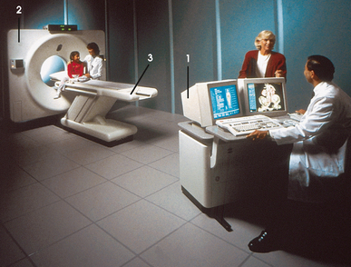
Fig. 31-13 Components of a CT scanner: 1, computer and operator’s console; 2, gantry; 3, patient table. (Courtesy GE Medical Systems, Waukesha, WI.)

COMPUTER

The computer provides the link between the CT technologist and the other components of the imaging system. The computer system used in CT has four basic functions: control of data acquisition, image reconstruction, storage of image data, and image display.

Data acquisition is the method by which the patient is scanned. The technologist must select among numerous parameters, such as scanning in the conventional or helical mode, before the initiation of each scan. During implementation of the data acquisition system (DAS), the computer is involved in sequencing the generation of x-rays, turning the detectors on and off at appropriate intervals, transferring data, and monitoring the system operation.

The reconstruction of a CT image depends on the millions of mathematic operations required to digitize and reconstruct the raw data. This image reconstruction is accomplished using an array processor that acts as a specialized computer to perform mathematic calculations rapidly and efficiently, freeing the host computer for other activities. Currently, CT units can acquire scans in less than 1 second and require only a few seconds more for image reconstruction.

The host computer in CT has limited storage capacity, so image data can be stored only temporarily. Other storage mechanisms are necessary to allow for long-term data storage and retrieval. After reconstruction, the CT image data can be transferred to another storage medium such as optical disks. CT studies can be removed from the limited memory of the host computer and stored independently, a process termed archiving.

The reconstructed images are displayed on a monitor. At this point, the technologist or physician can communicate with the host computer to view specific images; post images on a scout; or implement image manipulation techniques such as zoom, control contrast and brightness, and image analysis techniques.

GANTRY AND TABLE

The gantry is a circular device that houses the x-ray tube, DAS, and detector array. Helical CT units also house the continuous slip ring and high-voltage generator in the gantry. The structures housed in the gantry collect the necessary attenuation measurements to be sent to the computer for image reconstruction.

At the equipment-assembly level, drawing-controlled medical equipment sheet metal parts such as internal brackets, mounting plates, trays, and access panels can be designed around subsystem mounting and service-access requirements.

The x-ray tube used in CT is similar in design to the tubes used in conventional radiography, but it is specially designed to handle and dissipate excessive heat units created during a CT examination. Most CT x-ray tubes use a rotating anode to increase heat dissipation. Many CT x-ray tubes can handle around 2.1 million heat units (MHU), whereas advanced CT units can tolerate 4 to 5 MHU.

The detectors in CT function as image receptors. A detector measures the amount of radiation transmitted through the body and converts the measurement into an electrical signal proportional to the radiation intensity. The two basic detector types used in CT are scintillation (solid-state) and ionization (xenon gas) detectors. Current detectors use scintillation (solid-state) detectors.

The gantry can be tilted forward or backward up to 30 degrees to compensate for body part angulation. The opening within the center of the gantry is termed the aperture. Most apertures are about 28 inches (71.1 cm) wide to accommodate a variety of patient sizes as the patient table advances through it.

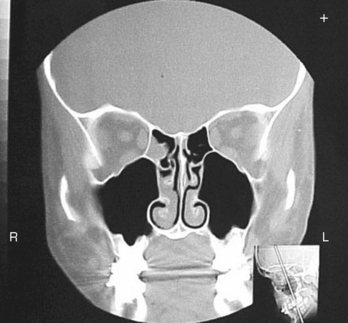
For certain head studies, such as studies of facial bones, sinuses, or the sella turcica, a combination of patient positioning and gantry angulation results in a direct coronal image of the body part being scanned. Fig. 31-14 shows a typical direct coronal image of the paranasal sinuses.

Fig. 31-14 Direct coronal of paranasal sinuses.

The table is an automated device linked to the computer and gantry. It is designed to move in increments (index) according to the scan program. The table is an extremely important part of a CT scanner. Indexing must be accurate and reliable, especially when thin slices (1 or 2 mm) are taken through the area of interest. Most CT tables can be programmed to move in or out of the gantry, depending on the examination protocol and the patient.

CT tables are made of wood or low-density carbon composite, both of which support the patient without causing image artifacts. The table must be very strong and rigid to handle patient weight and at the same time maintain consistent indexing. All CT tables have a maximum patient weight limit; this limit varies by manufacturer from 300 to 600 lb (136 to 272 kg). Exceeding the weight limit can cause inaccurate indexing; damage to the table motor; and even breakage of the tabletop, which could cause serious injury to the patient.

Accessory devices can be attached to the table for various uses. A special device called a cradle is used for head CT examinations. The head cradle helps hold the head still; because the device extends beyond the tabletop, it minimizes artifacts or attenuation from the table while the brain is being scanned. It can also be used in positioning the patient for direct coronal images.

OPERATOR’S CONSOLE

The operator’s console (Fig. 31-15 ) is the point from which the technologist controls the scanner. A typical console is equipped with a keyboard for entering patient data and a graphic monitor for viewing the images. Other input devices, such as a touch display screen and a computer mouse, may also be used. The operator’s console allows the technologist to control and monitor numerous scan parameters. Radiographic technique factors, slice thickness, table index, and reconstruction algorithm are some of the scan parameters that are selected at the operator’s console.

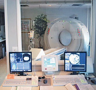
Fig. 31-15 CT operator’s console, workstation for three-dimensional image manipulation, and power injector control panel.

Before starting an examination, the technologist must enter the patient information. A keyboard is still necessary for some functions. Usually the first scan program selected is the scout program from which the radiographer plans the sequence of axial scans. An example of a typical scout image is seen in Fig. 31-3 . The operator’s console is also the location of the monitor, where image manipulation takes place. Most scanners display the image on the monitor in a 1024 matrix interpolated by the computer from the 512 reconstructed images.

One of the most important functions of the operator’s console is to initiate the process to store or archive the images for future viewing. To produce hard copies of images in the form of film, the most commonly used filming device is the laser printer. Most modern imaging departments now have picture archiving and communications systems (PACS) that are used to store and retrieve soft copy (digital) images.

OTHER COMPONENTS

Display monitor

For the CT image to be displayed on a monitor in a recognizable form, the digital CT data must be converted into a gray-scale image. This process is achieved by the conversion of each digital CT number in the matrix to an analog voltage. The brightness values of the gray-scale image correspond to the pixels and CT numbers of the digital data they represent.

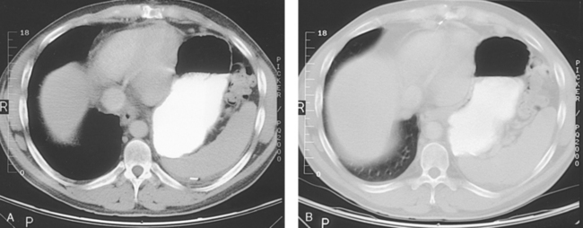
Because of the digital nature of the CT image data, image manipulation can be performed to enhance the appearance of the image. One of the most common image processing techniques is called windowing, or gray-level mapping. This technique allows the technologist to alter the contrast of the displayed image by adjusting the window width and window level. The window width is the range of CT numbers that are used to map signals into shades of gray. Basically, the window width determines the number of gray levels to be displayed in the image. A narrow window width means that there are fewer shades of gray, resulting in higher contrast. Likewise, a wide window width results in more shades of gray in the image, or a longer gray scale. The window level determines the midpoint of the range of gray levels to be displayed on the monitor. It is used to set the center CT number within the range of gray levels being used to display the image. The window level should be set to the CT number of the tissue of interest, and the window width should be set with a range of values that would optimize the contrast between the tissues in the image. Fig. 31-16 shows an axial image seen in two different windows: a standard abdomen window and a bone window adjusted for the spine.

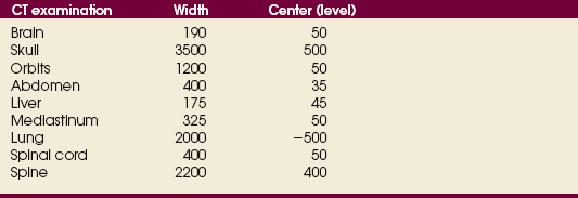
Fig. 31-16 A, Abdominal image, soft tissue window. B, Abdominal image, bone window.

The gray level of any image can be adjusted on the monitor to compensate for differences in patient size and tissue densities or to display the image as desired for the examination protocol. Examples of typical window width and level settings are listed in Table 31-2 . These settings are averages and usually vary by machine. The level, although an average, is approximately the same as the CT numbers expected for the tissue densities.

TABLE 31-2

Typical window settings

Workstation for image manipulation and multiplanar reconstruction

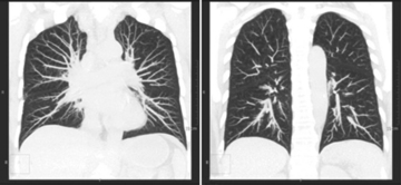
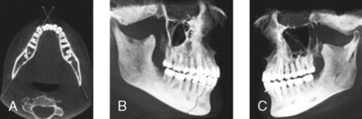
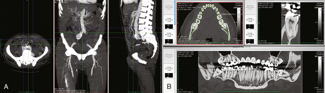
Another advantage of the digital nature of the CT image is the ability to reconstruct the axial images into coronal, sagittal, or oblique body planes without additional radiation to the patient. Image reconstruction in various planes is accomplished by stacking multiple contiguous axial images, creating a volume of data. Because the CT numbers of the image data within the volume are already known, a sectional image can be generated in any desired plane by selecting a particular plane of data. This postprocessing technique is termed multiplanar reconstruction (MPR). A coronal reconstruction from axial images is seen in Figs. 31-17 and 31-18 . Fig. 31-17 shows a coronal image of the abdomen (note the liver lesion), and Fig. 31-18 shows coronal images of the lungs displayed with a lung window width and window level. MPRs may also be performed in what is referred to as curved planar reformations to visualize structures better. Fig. 31-19 shows an axial image and oblique reformation of the mandible from the axial images

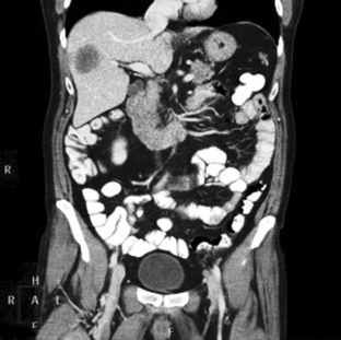
Fig. 31-17 Coronal reformatted image produced from axial images of abdomen and pelvis. (Courtesy Philips Medical Systems.)

Fig. 31-18 Coronal reformatted images produced from axial low-dose lung nodule study of the chest. Scans produced with Philips Brilliance iCT. (Courtesy Philips Medical Systems.)

Fig. 31-19 A, Axial mandible showing reconstruction planes. B, Oblique MPR left mandible (note fracture). C, Oblique MPR right mandible. (Courtesy Philips Medical Systems.)

Diagnostic Applications

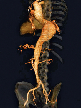
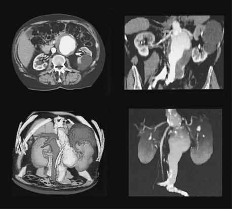
The original CT studies were used primarily for diagnosing neurologic disorders. As scanner technology advanced, the range of applications was extended to other areas of the body. The most commonly requested procedures involve the head, chest, and abdomen. CT is the examination of choice for head trauma; it clearly shows skull fractures and associated subdural hematomas. CT examinations of the head are one of the first tests performed on patients being evaluated for stroke or cerebrovascular accident where evidence of hemorrhage must be ruled out. CT imaging of the central nervous system can show infarctions, hemorrhage, disk herniations, craniofacial and spinal fractures, and tumors and other cancers. CT imaging of the body excels at showing soft tissue structures within the chest, abdomen, and pelvis. Among the abnormalities shown in this region are metastatic lesions, aneurysms (Fig. 31-20 ), abscesses, and fluid collections from blunt trauma.

Fig. 31-20 Three-dimensional abdominal aortic aneurysm (AAA).

CT is also used for numerous interventional procedures, such as abscess drainage, tissue biopsy (Fig. 31-21 ), and cyst aspiration. In addition, CT is used during radiofrequency ablations and cryoablations of tumors. Fig. 31-22 shows numerous structures and pathologic conditions identified by CT. Fig. 31-23 shows a liver lesion before radiofrequency ablation, during the procedure and after ablation.

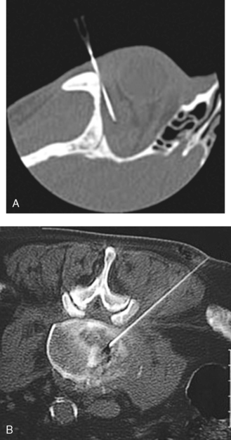
Fig. 31-21 A, Needle biopsy of orbital mass. B, Needle biopsy of infectious spondylitis of lumbar vertebral body.

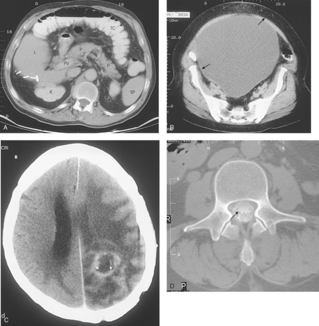
Fig. 31-22 A, Abdominal image showing transverse colon (TC) with air-fluid levels; liver (L), pancreas (P), spleen (SP), kidney (K), portal vein (PV), celiac trunk (CT), and splenic veins (SV) are shown with contrast medium. Surgical clips are seen in posterior liver. B, Abdominal image showing extremely large ovarian cyst (arrows). C, Brain image showing parietooccipital mass (arrow) with characteristic IV contrast ring enhancement (arrowhead). D, Image of L3 after myelography showing contrast material in thecal sac (arrow).

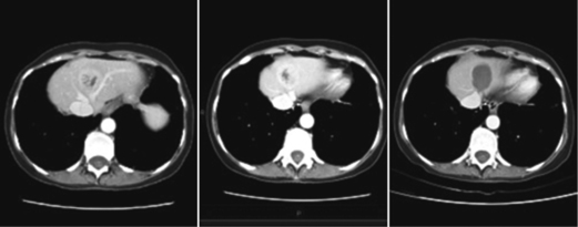
Fig. 31-23 Low-dose axial CT images from radiofrequency ablation study. Scans are before study (left), during study (middle), and after study (right). (Courtesy Philips Medical Systems.)

For any procedure, a protocol is required to maximize the amount of diagnostic information available. Specific examination protocols vary according to the needs of different medical facilities and physicians.

Contrast Media

Contrast media are used in CT examinations to help distinguish normal anatomy from pathology and to make various disease processes more visible. A contrast agent can be administered intravenously, orally, or rectally. Generally, intravenous (IV) contrast media are the same as media used for excretory urograms. Many facilities use nonionic contrast material for these studies because of the low incidence of reaction and known safety factors associated with nonionic contrast material. IV contrast media are useful for showing tumors within the head; Fig. 31-24 shows a brain scan with and without contrast media. The anterior lesion is evident in the unenhanced scan; in the enhanced scan, the tumor shows characteristic ring enhancement typical of tumors seen in CT scans. IV contrast media are also used to visualize vascular structures in the body.

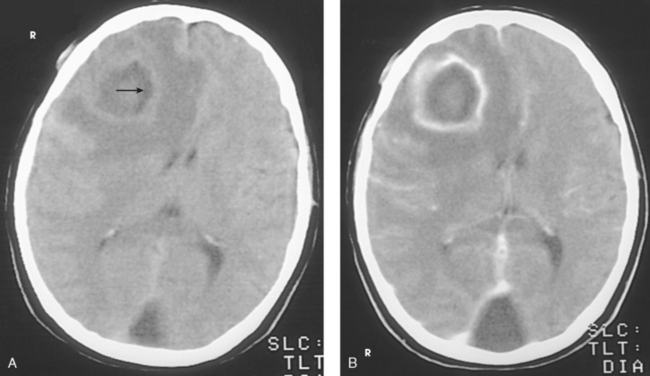
Fig. 31-24 A, Brain image without IV contrast agent showing lesion (arrow). B, Brain image with IV contrast agent.

IV contrast media should be used only with approval of the radiologist and after careful consideration of the patient’s medical and allergy history. The patient’s renal function must be evaluated before iodinated contrast material is given. Creatinine level and glomerular filtration rate are the most common laboratory values used to determine renal function. Many CT examinations can be performed without IV contrast material if necessary; however, the amount of diagnostic information available can be limited.

Oral contrast media must be used for imaging the abdomen. When given orally, the contrast material in the gastrointestinal tract helps differentiate between loops of bowel and other structures within the abdomen. An oral contrast medium is generally a 2% barium mixture. The low concentration prevents contrast artifacts but allows good visualization of the stomach and intestinal tract. An iodinated contrast material such as oral Hypaque can be used, but it must be mixed at low concentrations to prevent contrast artifacts. Rectal contrast medium is often requested as part of an abdominal or a pelvic protocol. Usually mixed in the same concentration as the oral contrast medium, the rectal contrast material is useful for showing the distal colon relative to the bladder and other structures of the pelvic cavity.

POWER INJECTOR USE FOR ADMINISTERING INTRAVENOUS CONTRAST MEDIA

Power injector use in CT examinations became mandatory when the first helical CT scanners were introduced. Faster delivery of IV contrast media became necessary with the reduced scan times used in helical CT. The advantage of power injector use is that a bolus injection of contrast medium can be delivered quickly, which provides for better contrast enhancement of structures and better opacification of the blood vessels. The use of power injectors also provides a means for reproducibility of examination parameters.

EQUIPMENT

Power injector equipment includes an injector assembly that is ceiling mounted next to the scanner or on a movable stand. The injector head typically has two syringes; however, some models may have only a single syringe delivery system. If the injector head is a double syringe system, each of the syringe controls is color-coded. The same color-coding system is seen on the injector control module that is next to the CT scan console. Programming the injector must be done at the control module, but operational buttons are located on the injector head and the control module.

The control module for the system is typically placed on or near the operator console of the scanner. Each injector system has controls for flow rate of the injection, pounds per square inch (psi) of pressure used for the injection, amount of contrast medium to be delivered, and time delays. Dual head systems have dual sets of controls for each syringe.

Special pressure syringes and pressure tubing must be used when injecting. The pressure injections must be closely monitored, and care must be taken that no air is in the syringe or tubing. The pressure syringes have oval etchings on the side of the syringe as a safety feature. If the syringe is full of contrast material, the oval etchings appear round when viewed through the syringe owing to light refraction. If there is no fluid present, the etchings remain oval in shape (Fig. 31-25 ).

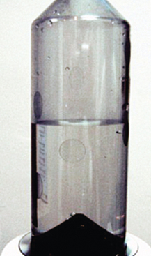
Fig. 31-25 CT pressure syringe partially filled with contrast material. Note oval etching above fluid level and round etching below fluid level.

Correct IV catheter size and placement is vital to the success of the CT examination. Catheters are typically placed in the arm veins in the antecubital fossa; however, veins lower in the forearm can also be used. Small veins should be avoided because of the pressures used when injecting. Catheter size depends on the type of CT examination being performed. A routine, non-CTA examination typically uses a 22-gauge angiocath with an injection rate of 2 mL/sec. A CTA study requires a larger bore 18-gauge to 20-gauge angiocath with an injection rate of 4 to 7 mL/sec.

PATIENT CARE AND INJECTION SAFETY

Patient positioning should be considered when placing the IV line. For many CT examinations, the patients must keep their arms resting above their head on a pillow or sponge during the examination. Care should be taken to make the patient as comfortable as possible while keeping their arms as straight as possible. The angiocatheter should not be placed in a site that would be bent when the patient elevates the arms above the head.

Proper placement of the angiocath should always be confirmed with a hand test injection of saline that mimics the injection rate of the examination. The ease of injection and the injection site should be observed and palpated during the test injection to confirm patency of the vein. The patient should be instructed to notify the CT technologist immediately if the patient experiences any pain or discomfort at the injection site during the procedure.

All connections between the angiocath, injector tubing, and syringe should be checked and tightened to prevent air from entering the IV line. The pressure syringe should be checked for air bubbles, and the etchings on the side of the syringe should be confirmed as round. The injected head and syringe should be pointed down to ensure that any potential air bubble would rise back into the syringe base and away from the IV line.

The patient should be instructed about the timing of the scan, the injection, and sensations of warmth and an odd taste caused by the dilation of the blood vessels. These sensations should be discussed with the patient, and the patient should be reassured that these are normal and fade quickly. The intensity of warmth and taste intensify as the injection amount and rate increase, so these are more intense for a patient having a CTA study.

If the patient complains of discomfort at or near the injection site, the injection should be terminated, and the patient should be checked for a contrast extravasation (contrast material leaking out of the vein). If there is any change in the appearance of the patient’s arm (swelling, discoloration), the radiologist should be notified immediately. The CT technologist should be familiar with the department policy for the treatment of extravasation, which typically includes cold and hot compresses and elevation of the arm.

Factors Affecting Image Quality

In CT, the technologist has access to numerous scan parameters that can have a dramatic effect on image quality. The four main factors contributing to image quality are spatial resolution, contrast resolution, noise, and artifacts.

SPATIAL RESOLUTION

Spatial resolution looks at the degree of blur or the ability to see the difference between two objects that are close together. The method most commonly used to evaluate spatial resolution is the number of line pairs per centimeter (lp/cm). The scan parameters that affect spatial resolution include section thickness, display FOV, matrix, and reconstruction algorithm/kernel. The detector aperture width is the most significant geometric factor that contributes to spatial resolution.

CONTRAST RESOLUTION

Contrast resolution is the ability to differentiate between small differences in density within the image. Currently, tissues with density differences of less than 0.5% can be distinguished with CT. The scan parameters that affect contrast resolution are slice thickness, reconstruction algorithm, image display, and x-ray beam energy. The size of the patient and the detector sensitivity also have a direct effect on contrast resolution.

TEMPORAL RESOLUTION

Temporal resolution is the ability of the CT system to freeze any motion of a scanned object. It is the shortest amount of time needed to acquire a complete data set. The use of CT in cardiac imaging requires high (shortest time) temporal resolution to decrease heart motion. Factors that improve temporal resolution include multidetector CT (i.e., 64-, 128-, 256-, 320-slice), tube/gantry rotation time, and the development of dual-source CT.

NOISE

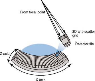
The most common cause of noise in CT is quantum noise. This type of noise arises from the random variation in photon detection. Noise in a CT image primarily affects contrast resolution. As noise increases in an image, contrast resolution decreases. Noise gives an image a grainy quality or a mottled appearance. Among the scan parameters that influence noise are matrix size, slice thickness, x-ray beam energy, and reconstruction algorithm. Scattered radiation and patient size also contribute to the noise of an image. New technology is available to prevent scatter radiation from hitting the detector. Fig. 31-26 shows the ClearRay Anti-Scatter Collimator (Philips Medical Systems), which greatly reduces noise and increases contrast resolution.

Fig. 31-26 Philips Medical Systems 2D Anti-scatter Grid, which can be focused for true three-dimensional cone-beam geometry. Scatter reduction improves low contrast resolution. (Courtesy Philips Medical Systems.)

ARTIFACTS

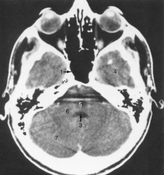
Metallic objects, such as dental fillings, pacemakers, and artificial joints, can cause starburst or streak artifacts, which can obscure diagnostic information. Dense residual barium from fluoroscopy examinations can cause artifacts similar to those caused by metallic objects. Many CT departments do not perform a CT examination in a patient until several days after barium studies to allow the body to eliminate the residual barium from the area of interest. Large differences in tissue densities of adjoining structures can cause artifacts that detract from image quality. Bone–soft tissue interfaces, such as occur with the skull and brain, often cause streak or shadow artifacts on CT images; these artifacts are referred to as beam hardening (Fig. 31-27 ).

Fig. 31-27 Streaking through the posterior fossa represents beam-hardening artifact. Normal appearance of the brain. 1, sphenoid sinus; 2, trigeminal ganglion; 3, fourth ventricle; 4, temporal lobe; 5, pons; 6, middle cerebellar peduncle; 7, cerebellar hemisphere.

OTHER FACTORS

Patient factors

Patient factors also contribute to the quality of an image. If a patient cannot or will not hold still, the scan is likely to be nondiagnostic. Body size also can have an effect on image quality. Large patients attenuate more radiation than small patients; this can increase image noise, detracting from overall image quality. An increase in milliampere-seconds (mAs) is usually required to compensate for large body size. This increase results in a higher radiation dose to the patient. Image quality factors under technologist control include slice thickness, scan time, scan diameter, and patient instructions. Slice thickness is usually dictated by image protocol. As in tomography, the thinner the slice thickness, the better the image-recorded detail. Thin-section CT scans, often referred to as high-resolution scans, are used to show structures better (Fig. 31-28 ).

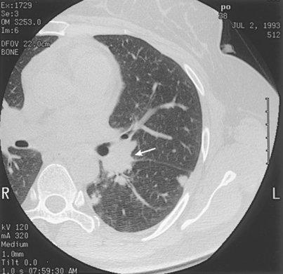
Fig. 31-28 High-resolution 1-mm slice using edge enhancement algorithm, showing nodule in left lung (arrow).

As in conventional radiography, patient instructions are a crucial part of a diagnostic examination. Explaining the procedure fully in terms that the patient can understand increases the level of compliance from almost any patient.

Scan times

Scan times are usually preselected by the computer as part of the scan program, but they can be altered by the technologist. When selecting a scan time, the technologist must take into account possible patient motion such as inadvertent body movements, breathing, or peristalsis. A good guideline is to choose a scan time that would minimize patient motion while providing a quality diagnostic image. When it is necessary to scan an uncooperative patient quickly, using the shortest scan time possible may allow the technologist to complete the examination, although the quality of the images obtained is likely to be compromised.

Scan diameter

The image that appears on the monitor depends on the scan diameter, also called scan FOV. The technologist can adjust the scan diameter to include the entire cross section of the body part being scanned or to include only a specified region within the part. The anatomy displayed is often referred to as the display FOV. Similar to scan time, scan diameter is usually preselected by the computer as part of a scan program, but it can also be adjusted as necessary by the technologist. For most head, chest, and abdomen examinations, the selected scan diameter includes all anatomy of the body part to just outside the skin borders. Certain examinations may require the scan diameter to be reduced to include specific anatomy, such as the sella turcica, sinuses, one lung, mediastinal vessels, suprarenal glands, one kidney, or the prostate.

Special Features

DYNAMIC SCANNING

One advantage of CT is that data can be obtained for image reconstruction by the computer. The scanner can be programmed to scan through an area rapidly. In this situation, raw data are saved, but image reconstruction after each scan is bypassed to shorten scan time.

Dynamic scanning is based on the principle that after contrast agent administration, different structures enhance at different rates. Dynamic scanning can consist of rapid sequential scanning at the same level to observe contrast material filling within a structure, such as is performed when looking for an aortic aneurysm. Another form of dynamic scanning is incremental dynamic scanning, which consists of rapid serial scanning at consecutive levels during the bolus injection of a contrast medium.

SINGLE SLICE SPIRAL OR HELICAL COMPUTED TOMOGRAPHY

Single slice spiral CT (SSCT) and helical CT are terms used to describe the current method of data acquisition in CT. During spiral CT, the gantry is rotating continuously while the table moves through the gantry aperture. The continuous gantry rotation combined with the continuous table movement forms the spiral path from which raw data are obtained one slice per revolution (Fig. 31-29 ). Slip-ring technology has made continuous rotation of the x-ray tube possible by eliminating the large high-voltage cables between the x-ray tube and the generators.

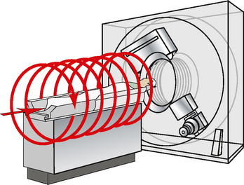
Fig. 31-29 Continuous gantry rotation combined with continuous table rotation, forming a spiral path of data.

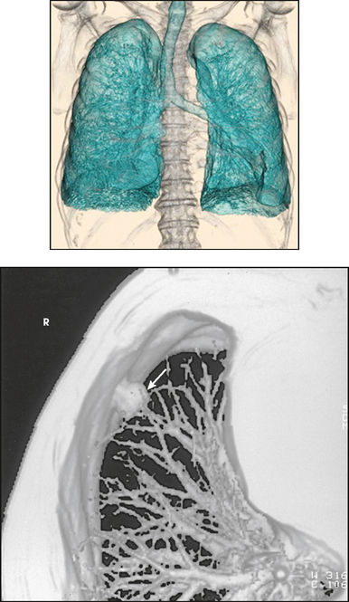
One of the unique features of spiral CT is that it scans a volume of tissue rather than a group of individual slices. This method makes it extremely useful for the detection of small lesions because an arbitrary slice can be reconstructed along any position within the volume of raw data. In addition, because a volume of tissue is scanned in a single breath, respiratory motion can be minimized. For a volume scan of the chest, such as shown in Fig. 31-30 , the patient is instructed to hold the breath, and a tissue volume of 24 mm is obtained in a 5-second spiral scan.

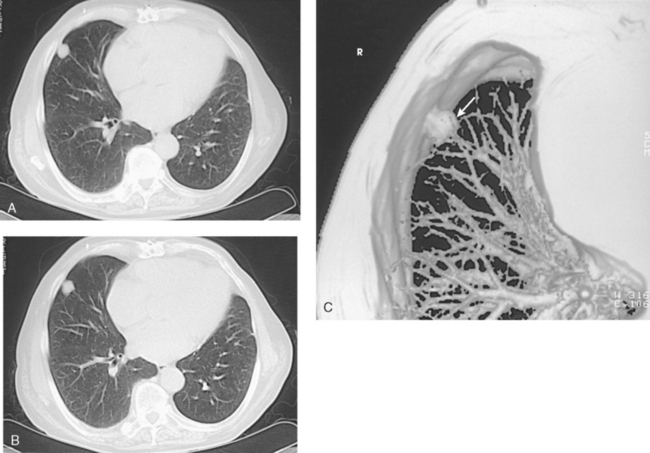
Fig. 31-30 A and B, Spiral images of lung showing lung nodule and associated vasculature. C, Three-dimensional reconstruction of lung nodule (arrow) after spiral scan. (Courtesy Siemens Medical Systems, Iselin, NJ.)

Two of the resultant images show a small lung nodule without breathing interference of image misregistration; a three-dimensional reconstruction of the lung clearly shows the pathologic condition. Spiral CT is especially useful when scanning uncooperative or combative patients; patients who cannot tolerate lying down for long periods; and patients who cannot hold still, such as pediatric patients or trauma patients. The use of spiral CT may decrease the amount of contrast medium necessary to visualize structures; this makes the examination safer and more cost-effective.

MULTISLICE SPIRAL OR HELICAL COMPUTED TOMOGRAPHY

Multislice helical CT (MSHCT) or multidetector CT (MDCT) systems incorporate a detector array that contains multiple rows of detector (channels) along the z axis compared with the single row of detectors in conventional spiral CT (SSCT). Each channel comprises numerous elements. In a “four-row” scanner, the detector array is connected to four data acquisition systems that generate four channels of data (Fig. 31-31 ). This type of detector array would allow a scan four times faster than the conventional single row spiral/helical scanner. Current technology detector arrays are 4, 8, 16, 32, 64, 128, 256, and 320 rows or channels. The increased width of the detector now requires the x-ray beam to be a cone-beam configuration compared with the fan beam used for SSCT. The 64-, 128-, 256-, and 320-row scanners are referred to as volume CT (VCT) systems because the amount of body section coverage in a single tube rotation. Figs. 31-32 and 31-33 were acquired on the Toshiba 320 row scanner in a single revolution. Fig. 31-32 is a three-dimensional volume rendering (VR) pediatric chest image acquired in 0.035 second. Fig. 31-33 shows a 16-cm volume coverage that allows for whole-brain perfusion imaging for evaluation of stroke. Cardiac imaging using VCT is a rapidly growing component of CT imaging. The advantages of MSHCT/MDCT include isotropic imaging and postprocessing, longer anatomic coverage, multiphase studies, faster examination times, and improved spatial resolution. The advancement of VCT, with increasing larger detector arrays, has provided unique clinical opportunities in diagnostic medicine. Fig. 31-34 compares the z-axis coverage of 64-, 128-, and 320-row detectors.

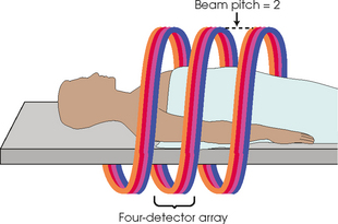
Fig. 31-31 Four-detector array with a beam pitch of 2.0 covers eight times the tissue volume of a single-slice spiral CT scan.

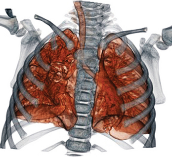
Fig. 31-32 Technology employing 320 detector rows makes it possible to scan an infant’s chest with fine detail, low radiation dose, and fast acquisition times. This image is a threedimensional VR acquired in a single rotation completed in 0.035 second. (Courtesy Toshiba America Medical Systems.)

Fig. 31-33 Whole-brain imaging is possible with 16 cm of volume coverage. This threedimensional VR whole-brain perfusion study shows evidence of acute stroke. (Courtesy Toshiba America Medical Systems.)

Fig. 31-34 Images show scan range for various row scanners. A, 64-row scanner. B, 128-row scanner. C, 320-row scanner. The 320-row scanner allows complete imaging of the cranial vessels with one table location. (Courtesy Toshiba America Medical Systems.)

COMPUTED TOMOGRAPHY ANGIOGRAPHY

CTA is an application of spiral CT that uses three-dimensional imaging techniques. With CTA, the vascular system can be viewed in three dimensions. The three basic steps required to generate CTA images are as follows:

1. Choice of parameters for IV administration of the bolus of contrast medium (i.e., injection rate, injection duration, and delay between bolus initiation and the start of the scan sequence)

2. Choice of spiral parameters to maximize the contrast medium in the target vessel (i.e., scan duration, collimation, and table speed)

3. Reconstruction of two-dimensional image data into three-dimensional image data

CTA has several advantages over conventional angiography. CTA uses spiral technology; an arbitrary image within the volume of data can be retrospectively reconstructed without exposing the patient to additional IV contrast medium or radiation. During postprocessing of the image data, overlying structures can be eliminated so that only the vascular anatomy is reconstructed. Finally, because CTA is an IV procedure that does not require arterial puncture, only minimal postprocedure observation is necessary.

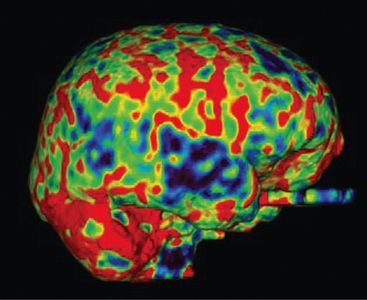
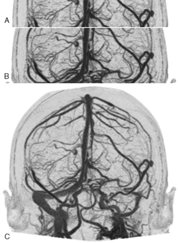
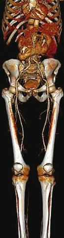
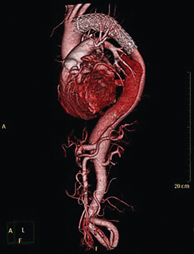
Currently, CTA is replacing angiography as a diagnostic tool for some studies. This is especially true in departments using multirow detectors that allow significantly faster scanning. Fig. 31-35 shows the vessels of the brain, whereas Fig. 31-36 shows the renal vessels in a three-dimensional format. The heart and coronary vessels are shown in Fig. 31-37 , and a graft is shown in Fig. 31-38 . Fig. 31-39 shows multiple reformations from a cardiac gated dose reduction method performed on a Philips Medical 256-row scanner. Fig. 31-40 is a brain perfusion study showing significant vascular changes on a patient with an acute stroke.

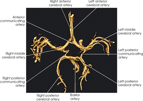
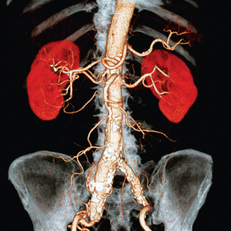
Fig. 31-35 Color CT angiography of circle of Willis.

Fig. 31-36 Color CT angiography in three-dimensional format. (Courtesy Toshiba America Medical Systems.)

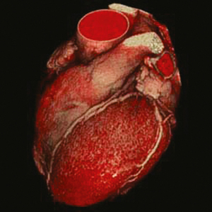
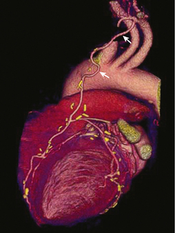
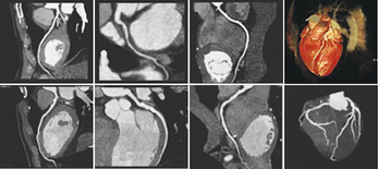
Fig. 31-37 Color three-dimensional cardiac CTA.

Fig. 31-38 Color three-dimensional cardiac CTA with graft (arrows).

Fig. 31-39 Prospectively gated CT angiograms. Low-dose studies performed with Philips Step and Shoot Cardiac software that has arrhythmia detection that stops scans until ECG stabilizes. (Courtesy Philips Medical Systems.)

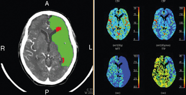
Fig. 31-40 CT brain perfusion study with brain perfusion parameter maps (right four images) and summary map overlays (left) showing areas of ischemic penumbra (green) and infarct (red). Images were acquired using a lower dose protocol on a Philips Brilliance CT scanner. (Courtesy Philips Medical Systems.)

THREE-DIMENSIONAL IMAGING

A rapidly expanding area of CT is three-dimensional imaging. This is a postprocessing technique that is applied to raw data to create realistic images of the surface anatomy to be visualized. The introduction of advanced computers and faster software programs has dramatically increased the applications of three-dimensional imaging. The common techniques used in creating three-dimensional images include maximum intensity projection (MIP), shaded surface display (SSD), and volume rendering (VR). All techniques use three initial steps to create the three-dimensional images from the original CT data:

1. Construction of a volume of threedimensional data from the original two-dimensional CT image data. This same process is used in MPR.

2. Segmentation to crop or edit the target objects from the reconstructed data. This step eliminates unwanted information from the CT data.

3. Rendering or shading to provide depth perception to the final image.

Maximum intensity projection

MIP consists of reconstructing the brightest pixels from a stack of two-dimensional or three-dimensional image data into a three-dimensional image. The data are rotated on an arbitrary axis, and an imaginary ray is passed through the data in specific increments. The brightest pixel found along each ray is mapped into a gray-scale image. MIP is commonly used for CTA.

Shaded surface display

SSD provides a three-dimensional image of the surface of a particular structure. After the original two-dimensional data are reconstructed into three-dimensional data, the different tissue types within the image need to be separated. This process, called segmentation, can be performed by drawing a line around the tissue of interest or, more commonly, by setting threshold values. A threshold value can be set for a particular CT number; the result is that any pixel having an equal or greater CT number than the threshold value would be selected for the three-dimensional image. When the threshold value is set and the data are reconstructed into a threedimensional image, a shading technique is applied. The shading or rendering technique provides depth perception in the reconstructed image.

Volume rendering

VR techniques incorporate the entire volume of data into a three-dimensional image by summing the contributions of each voxel along a line from the viewer’s eye through the data set. This results in a three-dimensional image in which the dynamic range throughout the image is preserved. Rather than being limited to surface data, a VR image can display a wide range of tissues that accurately depict the anatomic relationships between vasculature and viscera. Because VR incorporates and processes the entire data set, much more powerful computers are required to reconstruct three-dimensional VR images at a reasonable speed.

Referring physicians and surgeons use three-dimensional images to correlate CT images clinically to the actual anatomic contours of their patients (Fig. 31-41 ). These reconstructions are especially useful in surgical procedures. Three-dimensional reconstructions are often requested as part of patient evaluation after trauma and for presurgical planning. Fig. 31-42 shows examples of the three common three-dimensional rendering techniques.

Fig. 31-41 A, MPR reconstruction of abdominal aorta. B, Curved MPR of mandible.

Fig. 31-42 Common three-dimensional rendering techniques used in CT. (Courtesy Elicit, Hackensack, NJ.)

RADIATION TREATMENT PLANNING

Radiation therapy has been used for nearly as long as radiology has been in existence. The introduction of CT has had a major impact on radiation treatment planning. The use of spiral CT in conjunction with MPR provides a three-dimensional approach to radiation treatment planning. This method helps the dosimetrist plan treatment so that the radiation dose to the target is maximized and the dose to normal tissue is minimized. The three-dimensional simulation software offers the following: volumetric, high-precision localization; calculation of the geometric center of the defined target; patient marking systems; and virtual simulators capable of producing digitally reconstructed radiographs in real time. With the new, specially designed software, a single CT simulation procedure can replace a total of three procedures (one conventional CT scan and two conventional simulations) for radiation treatment planning (Fig. 31-43 ).

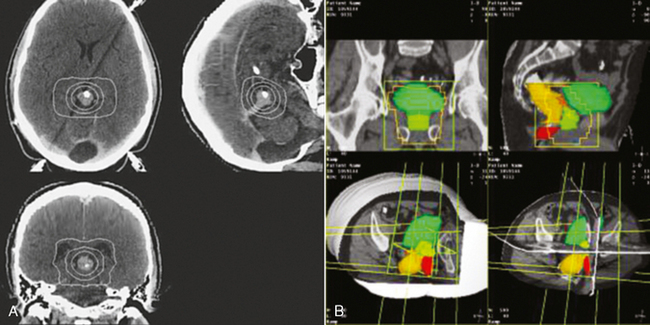
Fig. 31-43 A, Brain localization in three planes. B, Three-dimensional prostate therapy localization.

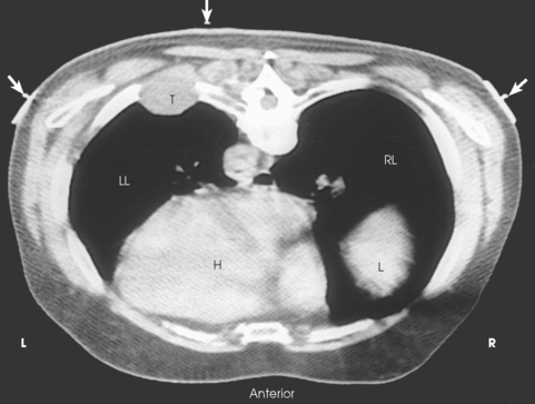
If the CT system is being used for radiation treatment planning, the standard curved couch should not be used. Instead, a flat board should be placed on the couch. In this way, the actual therapy delivery can be simulated more accurately. Fig. 31-44 shows the external skin markers and structures that would be in the beam’s path.

Fig. 31-44 Patient in prone position for radiation treatment planning. Radiopaque markers (arrows) show location of treatment field skin marks: tumor (T), heart (H), liver (L), right lung (RL), and left lung (LL).

PET/CT SCANNERS

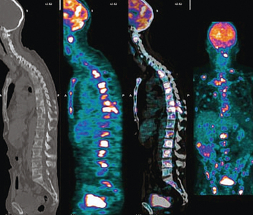
When a CT scanner are coupled with a positron emission tomography (PET) scanner, it is referred to as a PET/CT scanner. The PET/CT scanner comprises two scanners in close proximity to each other with a single patient couch that travels between the two scanners. In some scanner configurations, there is a small gap between the scanner housings; in other configurations, the scanner appears to be a single unit. Current PET/CT scanners are typically third-generation scanners and incorporate the latest in detector technology. Most modern PET/CT scanners incorporate 8-, 16-, and 64-row detectors. PET/CT is discussed in more detail in Chapter 34 ; the scanners are typically housed in the nuclear medicine department instead of the CT department. The CT scanner is used for attenuation correction and anatomic correlation for the functional PET scans. Many patients require a more detailed diagnostic CT examination as well, however, which has required nuclear medicine technologists to obtain additional training. Fig. 31-45 shows sagittal reconstructed CT spine images and the corresponding PET images and PET/CT fusion image.

Fig. 31-45 Sagittal reformatted CT scan (far left), sagittal PET (second from left), PET/CT fusion image (second from right) and coronal PET (far right).

QUALITY CONTROL

The goal of any quality assurance program in CT is to ensure that the system is producing the best possible image quality with the minimum radiation dose to the patient. A CT system is a complex combination of sensitive and expensive equipment that requires systematic monitoring for performance and image quality. Most CT systems require weekly or biweekly preventive maintenance to ensure proper operation.

Preventive maintenance is usually performed by a service engineer from the manufacturer or a private company. Increasingly, the technologist is being assigned the responsibility of performing and documenting routine quality assurance tests. Many technologists routinely perform daily test scans on a water phantom to measure the consistency of the CT numbers and to record the standard deviation. As data are recorded over time, the CT scanner’s current operating condition and its performance over longer time periods can be evaluated. Many units are also capable of air calibrations, which do not require the water phantom and can be performed between patients for unit self-calibration.

A CT phantom is typically multisectioned and is constructed from plastic cylinders, with each section filled with test objects designed to measure the performance of specific parameters. Some phantoms are designed to allow numerous parameters to be evaluated with a single scan. The recommended quality assurance tests for evaluating routine performance include contrast scale and mean CT number of water, high-contrast resolution, low-contrast resolution, laser light accuracy, noise and uniformity, slice thickness, and patient dose.

Computed Tomography and Radiation Dose

Calculating the radiation dose received during CT examinations presents a unique set of circumstances. Typically, radiation received during radiologic examinations comes from a fixed source with delivery to the patient in one or two planes (e.g., AP and lateral views). These exposure parameters typically produce a much higher entrance skin dose than the exit skin dose, which creates a large dose gradient across the patient. In contrast, CT exposures (helical/spiral) come from an essentially continuous source that rotates 360 degrees around the patient. This results in a radially symmetric radiation dose gradient within the patient. Equipment manufacturers are developing new wedge (bow-tie) filters to reduce patient dose. Fig. 31-46 shows the SmartShape wedge from Philips Medical Systems. Note the dose reduction shown on the center image when the appropriate filter is applied.

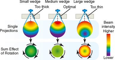
Fig. 31-46 Diagram represents selectable bow-tie filters that reduce patient dose and improve image quality. These are referred to as SmartShape wedges on the Philips Brilliance iCT scanner. Note how correct wedge selection affects patient dose. Wedges are typically small (infants 0 to 18 months), medium (cardiac), and large (adult head and body). Wedge selection is built into scan protocols. (Courtesy Philips Medical Systems.)

Measurements of CT dose are typically performed using a circular CT dosimetry phantom that is made of polymethyl methacrylate (PMMA) with implanted thermoluminescent dosimeters (TLDs). The TLDs are positioned 1 cm below the surface around the periphery of the phantom and at the center (isocenter). The typical phantom sizes are 32 cm for body calculations and 16 cm for head calculations. For a single axial scan location (one full rotation of the tube, no table movement), the typical dose for the body phantom is 20 mGy at the periphery and 10 mGy at the isocenter. The typical dose for the head phantom is higher at 40 mGy at the periphery and 40 mGy at the isocenter. See Fig. 31-47 for the body and Fig. 31-48 for the head. Dose is size dependent (e.g., dose differs depending on head scan or body scan and whether the patient is a child or adult).

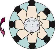
Fig. 31-47 CT dose profile for body. (Data from McNitt-Gray MF: AAPM/RSNA physics tutorial for residents: topics in CT. Radiation dose in CT, RadioGraphics 22:1541, 2002.)

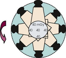
Fig. 31-48 CT dose profile for head. (Data from McNitt-Gray MF: AAPM/RSNA physics tutorial for residents: topics in CT. Radiation dose in CT, RadioGraphics 22:1541, 2002.)

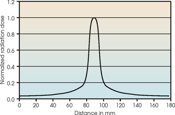
Another component of dose to the patient is distribution of absorbed dose along the length of the patient from one single scan (full rotation at one table location). The radiation dose profile (Fig. 31-49 ) is not limited just to the slice location; the “tails” of the dose profile contribute to the absorbed dose outside of the primary beam. The size of the contribution to dose from the adjacent sections is directly related to the spacing of the slices and the width and shape of the radiation profile. The first method used to describe dose as a result of multiple scan locations was the multiple scan average dose (MSAD). MSAD described average dose resulting from scans over an interval length on the patient. Next was the computed tomography dose index (CTDI), which was calculated using a normalized beam width and a standard of 14 contiguous axial slices. This method required a dose profile measured with TLDs or film, neither of which was convenient. To overcome the measurement limitations, another dose index, the CTDI₁₀₀, was developed. This dose index allowed profile calculations along the full length (100 mm) of a pencil ionization chamber and did not require nominal section widths. To provide a weighted average of the center and peripheral contributions, CTDI_w was created. The final descriptor is CTDI_vol, which accounts for the helical pitch or axial scan spacing that is used for a specific protocol. The most common reporting method of dose reporting on the present scanners is the dose-length product (DLP). This is the CTDI_vol multiplied by the length of the scan (cm). It is reported in mGy/cm.

Fig. 31-49 Single-slice CT dose profile.

Patient dose must be a part of the permanent record for each examination. Each manufacturer displays dose parameters in various ways. Fig. 31-50 is an example of how Philips Medical Systems displays dose information (note parameters within blue box just above the “go” button).

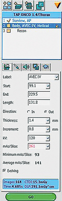
Fig. 31-50 Dose amounts must be reported for every series and protocol performed. Each manufacturer displays information differently. Note CTDI and DLP displayed inside the blue box. (Courtesy Philips Medical Systems.)

ESTIMATING EFFECTIVE DOSE

Effective dose takes into account where the radiation dose is being absorbed (e.g., which tissue or organ has absorbed the radiation). The weighting factors are set for each radiosensitive organ by the International Commission on Radiological Protection (ICRP) (available at www.ICRP.org ). Effective dose is measured in sieverts (Sv) or rems (100 rem = 5 1 Sv). The effective dose is determined by multiplying the DLP by a region-specific conversion factor. The conversion factors are 0.017 mSv/mGy/cm for chest imaging, 0.019 mSv/mGy/cm for pelvis imaging, and 0.0023 mSv/mGy/cm for head imaging. The conversion factor for head scans is considerably less because there are fewer radiosensitive organs that are irradiated. (The DLP for a given chest examination is 375 mGy; the resulting estimated effective dose is 375 multiplied by 0.017, which equals 6.4 mSv.)

Factors That Affect Dose

The factors that directly influence the radiation dose to the patient are beam energy (kVp), tube current (mA), rotation or exposure time (seconds), section or slice thickness (beam collimation), object thickness and attenuation (size of patient, pediatric vs. adult), pitch or section spacing (table distance traveled in one 360degree rotation), dose reduction techniques (mA modulation), and distance from the tube to isocenter. Patient shielding in the scan area is now possible with bismuth-filled shields, which yield little image artifact but provide 50% to 60% dose reduction. Adult breast shields, various sized pediatric breast shields, thyroid shields, and eye shields are presently available.

Fig. 31-51 shows a technique of mA modulation that uses an AP and lateral scout image to calculate patient thickness, which results in automatic mA adjustments during the scan (see red line). New “selectable” filters (Fig. 31-52 ) have been developed that allow different filter applications based on body section or patient age or size. These filters can reduce dose by nearly 30% when using 120 kVp and 45% when using 80 kVp.

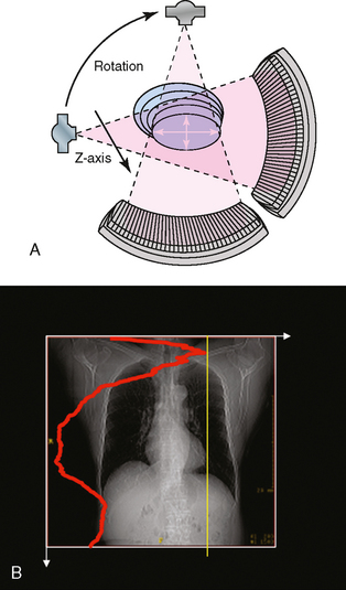
Fig. 31-51 A, AP and lateral scout images performed for mA modulation calculations. Note thickness difference A/P versus R/L. B, Philips DoseRight automated tube current selection (ACS). Red line shows z-axis dose modulation. Note technique increase in shoulder and abdomen region and technique decrease in lung region. (Courtesy Philips Medical Systems.)

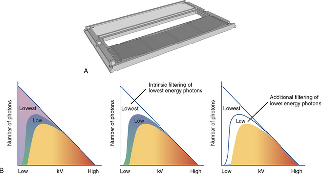
Fig. 31-52 A, IntelliBeam adjustable filter that controls beam hardness (quality). Filters are used in conjunction with wedges to reduce patient dose. B, Graph showing decrease in dose owing to elimination of low-energy photons (far right diagram). (Courtesy Philips Medical Systems.)

Beam collimation (slice thickness) varies in single-detector scanners and multidetector scanners. Beam collimation for single-detector systems has minimal effect on dose; however, this is not the case for multidetector scanners. These scanners have multiple ways to scan and reconstruct images. A multidetector scanner can perform axial scans of 4 × 1.25 mm (5-mm beam width, 1.25-mm slice reconstruction), 4 × 2.5 mm (10-mm beam width, 2.25-mm slice reconstruction), and 4 × 5.0 mm (20-mm beam width, 5.0-mm slice reconstruction). When all other parameters are kept constant, there are significant differences in dose. Beam collimation, not reconstruction thickness, results in a difference in some cases of 55% in the head phantom and 65% in the body phantom when comparing single-detector versus multidetector scanners. See Table 31-3 for single-detector imaging dose chart, Table 31-4 for multidetector imaging dose chart, and Table 31-5 for multidetector imaging with new dose reduction techniques.

TABLE 31-3

Single-detector doses

TABLE 31-4

Multidetector doses

TABLE 31-5

Low-dose protocols (Philips Brilliance iCT)

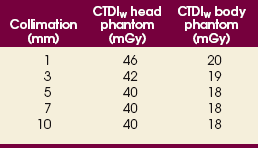
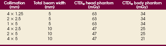
Patient size must be considered carefully when setting up scan parameters. A small adult or pediatric patient absorbs less of the entrance radiation than a larger patient. This results in the exit radiation dose of higher intensity, which results in a more uniform dose distribution. The distribution is nearly equal at all locations in a 16-cm phantom, a factor of two times greater. A larger patient has a much lower exit radiation dose, which reduces the total dose distribution in a 32-cm phantom.

Comparison of Computed Tomography and Magnetic Resonance Imaging

As CT was developing and advancing into a significant diagnostic modality, magnetic resonance imaging (MRI) was also progressing. Similar to CT, MRI was first used to image the brain; whole-body scans were developed shortly afterward. As MRI advanced and the quality of the images improved, it became apparent that MRI images exhibited better low-contrast resolution than CT images. Brain soft tissue detail is not shown as well with CT as with MRI performed at approximately the same level (Fig. 31-53 ).

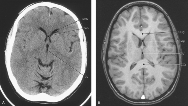
Fig. 31-53 A, Axial CT scan of lateral ventricles (LVah). B, Axial MRI scan of corpus callosum. (From Kelley LL, Petersen CM: Sectional anatomy for imaging professionals, St Louis, ed 2, 2007, Mosby.)

The initial introduction of MRI raised concerns that CT scanners would become obsolete. Each modality has been found to have unique capabilities, however. CT and MRI are useful for different clinical applications. As previously mentioned, CT does not show soft tissue as well as MRI; however, CT shows bony structures better than MRI.

Patients often have ferrous metal within their bodies. Such patients cannot always be scanned by MRI. CT is one option for these patients. The CT scanner does not affect metal in a patient, but metal can cause artifacts on CT images when the metal lies within the scan plane.

Many patients (especially pediatric and trauma patients) are extremely claustrophobic, combative, or uncooperative. CT is useful for scanning these patients quickly and easily because of the short gantry length, relatively large aperture, and short scan times.

Because equipment costs are less and a greater number of procedures can be accomplished per day, CT often is a less costly examination than MRI. Physicians have found that CT and MRI can be complementary examinations. In many situations, both examinations are ordered to provide as much diagnostic information as possible.

Future Considerations

In the last 5 years, CT has significantly increased its diagnostic capabilities. The development of multirow detectors was central to the advancement of CT as a discipline. With the rapid advancements in technology, the CT technologist has an increased responsibility to understand contrast dynamics and the spiral scan parameters of pitch, collimation, scan timing, and table speed.

Advancements in dose reduction, spatial resolution, and temporal resolution will continue. Manufacturers are working hard to improve ALARA (as low as reasonably achievable) practices and to meet or exceed the standards published by Image Gently, The Alliance for Radiation Safety in Pediatric Imaging (imagegently.org ).

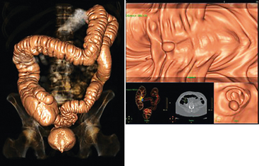
Advances in computing power and design have provided workstations that can generate three-dimensional models, rotate the models along any axis, and display the models with varying parameters (Figs. 31-54 and 31-55 ). Digital subtraction CT, multimodality image superimposition, and translucent shading of soft tissue structures are some newer applications. Physicians can manipulate the anatomy on virtual reality and other graphics platforms. Virtual colonoscopy (Fig. 31-56 ), virtual bronchoscopy, virtual cholangiopancreatography, and virtual labyrinthoscopy (inner ear) are continuing to evolve. Virtual dissection of the colon is being investigated as a replacement for invasive colonoscopy procedures. Multienergy and flat panel detectors are in development. As higher quality images increase the accuracy of diagnosis and treatment, patient care will be improved. Because of the superb diagnostic information and cost-effectiveness that CT provides, this imaging modality will continue to be a highly respected diagnostic tool.

Fig. 31-54 Full-body three-dimensional reconstruction from 64-row CT scanner.

Fig. 31-55 Aortic arch stent shown on 500-mm three-dimensional reconstruction. (Courtesy Philips Medical Systems.)

Fig. 31-56 CT colonography. (Courtesy Philips Medical Systems.)

Definition of Terms

air calibration Scan of air in gantry; based on a known value of −1000 for air, the scanner calibrates itself according to this density value relative to actual density value measured.

algorithm Mathematic formula designed for computers to carry out complex calculations required for image reconstruction; designed for enhancement of soft tissue, bone, and edge resolution. Also referred to as kernel.

anisotropic spatial resolution Spatial resolution of a voxel in which all three axes of the volume element are not equal. Slice thickness is not equal to pixel size.

aperture Opening of the gantry through which patient passes during scan.

archiving Storage of CT images on long-term storage device such as cassette tape, magnetic tape, or optical disk.

artifact Distortion or error in image that is unrelated to subject being studied.

attenuation Coefficient CT number assigned to measured remnant radiation intensity after attenuation by tissue density.

axial Describes plane of image as presented by CT scan; same as transverse.

bolus Preset amount of radiopaque contrast medium injected rapidly per IV administration to visualize high-flow vascular structures, usually in conjunction with dynamic scan; most often injected using a pressure injector.

channel In multidetector CT, multiple rows of detectors (channels) are arranged along the longitudinal (z) axis of the patient. Each detector row (channel) consists of numerous elements.

computed tomography (CT) X-ray tube and detector assembly rotating 360 degrees around a specified area of the body; also called CAT (computed axial tomography) scan.

computed tomography dose index (CTDI) Radiation dose descriptor calculated with normalized beam widths for 14 contiguous sections or slices.

computed tomography dose index₁₀₀ (CTDI₁₀₀) Radiation dose descriptor calculated with the full length of a 100-mm pencil ionization chamber. Measures larger scan distances than CTDI, but only one location is calculated.

computed tomography dose index_vol (CTDI_vol) Radiation dose descriptor that takes into account the parameters that are related to a specific imaging protocol. Considers helical pitch or axial scan spacing in its calculation. More accurate measure of dose per protocol.

computed tomography dose index_w (CTDI_w) Radiation dose descriptor that provides a weighted average of the center and peripheral contributions to dose within the scan plane. More accurate than CTDI₁₀₀ owing to calculations from more than one location.

CT angiography Use of volumetric CT scanning with spiral technique to acquire image data that are reconstructed into three-dimensional CT angiograms.

CT number Arbitrary number assigned by computer to indicate relative density of a given tissue; CT number varies proportionately with tissue density; high CT numbers indicate dense tissue, and low CT numbers indicate less dense tissue. All CT numbers are based on the density of water, which is assigned a CT number of 0. Also referred to as a Hounsfield unit.

contrast resolution Ability to differentiate between small differences in density within the image.

curved planar reformations Postprocessing technique applied to stacks of axial image data that can be reconstructed into irregular or oblique planes.

data acquisition system (DAS) Part of detector assembly that converts analog signals to digital signals that can be used by the CT computer.

detector Electronic component used for radiation detection; made of either high-density photo reactive crystals or pressurized stable gases.

detector assembly Electronic component of CT scanner that measures remnant radiation exiting the patient, converting the radiation to an analog signal proportionate to the radiation intensity measured.

direct coronal Describes position used to obtain images in coronal plane; used for head scans to provide images at right angles to axial images; patient is positioned prone for direct coronal images and supine for reverse coronal images.

dose length product (DLP) Commonly reported dose descriptor on CT scanners. Calculated by multiplying the CTDI_vol by the length of the scan (cm). DLP = 5 CTDI_vol × scan length.

dynamic scanning Process by which raw data are obtained by continuous scanning; images are not reconstructed but are saved for later reconstruction; most often used for visualization of high-flow vascular structures; can be used to scan a uncooperative patient rapidly.

field of view (FOV) Area of anatomy displayed on the monitor; can be adjusted to include entire body section or a specific part of the patient anatomy being scanned.

gantry Part of CT scanner that houses x-ray tube, cooling system, detector assembly, and DAS; often referred to as the “doughnut” by patients.

generation Description of significant levels of technologic development of CT scanners; specifically related to tube detector movement.

gray-scale image Analog image whereby each pixel in the image corresponds to a particular shade of gray.

helical CT Data acquisition method that combines continuous gantry rotation with continuous table movement to form a helical path of scan data; also called spiral CT.

high-resolution scans Use of scanning parameters that enhance contrast resolution of an image, such as thin slices, high matrices, high-spatial frequency algorithms, and small-display FOV.

host computer Primary link between system operator and other components of imaging system.

Hounsfield unit (HU) Number used to describe average density of tissue; term is used interchangeably with CT number; named in honor of Hounsfield, who is generally given credit for development of the first clinically viable CT scanner.

image misregistration Image distortion caused by combination of table indexing and respiration; table moves in specified increments, but patient movement during respiration may cause anatomy to be scanned more than once or not at all.

index Table movement; also referred to as table increments.

isotropic spatial resolution Spatial resolution of a voxel in which all three axes of the volume element are equal. Slice thickness is equal to pixel size.

mapping Assignment of appropriate gray level to each pixel in an image.

matrix Mathematical formula for calculation made up of individual cells for number assignment; CT matrix stores a CT number relative to the tissue density at that location; each cell or “address” stores one CT number for image reconstruction.

maximum intensity projection (MIP) Reconstruction of brightest pixels from stack of image data into a threedimensional image.

multiplanar reconstruction (MPR) Postprocessing technique applied to stacks of axial image data that can be reconstructed into other orientations or imaging planes.

multiple scan average dose (MSAD) Dose descriptor that calculates average dose resulting from a series of scans over an interval length of scans.

noise Random variation of CT numbers around some mean value within a uniform object; noise produces a grainy appearance in the image.

partial volume averaging Calculated linear attenuation coefficient for a pixel that is a weighted average of all densities in the pixel; the assigned CT number and ultimately the pixel appearance are affected by the average of the different densities measured within that pixel.

pixel (picture element) One individual cell surface within an image matrix used for image display.

postprocessing techniques Specialized reconstruction techniques that are applied to CT images to display the anatomic structures from different perspectives.

primary data CT number assigned to the matrix by the computer; the information required to reconstruct an image.

protocol Instructions for CT examination specifying slice thickness, table increments, contrast administration, scan diameter, and any other requirements specified by the radiologist.

quantum noise Any noise in the image that is a result of random variation in the number of x-ray photons detected.

real time Ability to process or reconstruct incoming data in milliseconds.

reconstruction Process of creating a digital image from raw data.

region of interest (ROI) Measurement of CT numbers within a specified area for evaluation of average tissue density.

rendering Process of changing the shading of a three-dimensional image; commonly used to increase depth perception of an image.

retrieval Reconstruction of images stored on long-term device; can be done for extra film copies or when films are lost.

scan Actual rotation of x-ray tube around the patient; used as a generic reference to one slice or an entire examination.

scan diameter Also referred to as the zoom or focal plane of a CT scan; predetermined by the radiographer to include the anatomic area of interest; determines FOV.

scan duration Amount of time used to scan an entire volume during a single spiral scan.

scan time X-ray exposure time in seconds.

segmentation Method of cropping or editing target objects from image data.

shaded surface display (SSD) Process used to generate three-dimensional images that show the surface of a three-dimensional object.

shading Postprocessing technique used in three-dimensional reconstructions to separate tissues of interest by applying a threshold value to isolate the structure of interest.

slice One scan through a selected body part; also referred to as a cut; slice thickness can vary from 0.35 mm to 1 cm, depending on the examination.

slip ring Low-voltage electrical contacts within the gantry designed to allow continuous rotation of an x-ray tube without the use of cables connecting internal and external components.

spatial resolution Ability to identify visibly anatomic structures and small objects of high contrast.

spiral CT Scanning method that combines a continuous gantry rotation with a continuous table movement to form a spiral path of scan data; also called helical CT.

streak artifact Artifact created by high-density objects that result in an arc of straight lines projecting across the FOV from a common point.

system noise Inherent property of a CT scanner; the difference between the measured CT number of a given tissue and the known value for that tissue; most often evaluated through the use of water phantom scans.

table increments Specific amount of table travel between scans; can be varied to move at any specified increment; most protocols specify from 1 mm to 20 cm, depending on type of examination; also referred to as indexing.

table speed Longitudinal distance traveled by the table during one revolution of the x-ray tube.

temporal resolution Ability of CT system to freeze motions of the scanned object; the shortest amount of time needed to acquire a complete data set.

threshold value CT number used in defining the corresponding anatomy that comprises a three-dimensional object; any pixels within a three-dimensional volume having the threshold value (CT number) or higher would be selected for the three-dimensional model.

useful patient dose Radiation dose received by the patient that is actually and converted into an image.

voxel (volume element) Individual pixel with the associated volume of tissue based on the slice thickness.

window Arbitrary numbers used for image display based on various shades of gray; window width controls the overall gray level and affects image contrast; window level (center) controls subtle gray images within a certain width range and ultimately affects the brightness and overall density of an image.

Selected bibliography

Bushong, SC. Radiologic science for technologists: physics, biology, and protection, ed 9. St Louis: Mosby, 2009.

Griffey, RT, Sodickson, A. Cumulative radiation exposure and cancer risk estimates in emergency department patients undergoing repeat or multiple CT. AJR Am J Roentgenol. 2009;192:887.

Haaga, JR, et al. ed 5. CT and MRI of the whole body, vols I and II.. Mosby: St Louis, 2009.

Image Gently, The Alliance for Radiation Safety in Pediatric Imaging Standards, Available at imagegently.org.

Joemai, RM, et al. Assessment of patient and occupational dose in established and new applications of MDCT fluoroscopy. AJR Am J Roentgenol. 2009;192:881.

Seeram, E. Computed tomography: physical principles, clinical applications, and quality control, ed 3. St Louis: Saunders, 2009.

^*Almost all italicized words on the succeeding pages are defined at the end of this chapter.

COMPUTED TOMOGRAPHY

GAYLE K. WRIGHT and MICHAEL L. GREY

OUTLINE

Basic Computed Tomography Examination Protocols

Fundamentals of Computed Tomography

Fig. 31-1 CT scanner provides cross-sectional images by rotating around the patient.

Computed Tomography and Conventional Radiography

Fig. 31-2 Conventional radiograph superimposes anatomy and yields one diagnostic image with fixed density and contrast.

Fig. 31-3 Digital kidney, ureter, and bladder (KUB).

Historical Development

Fig. 31-6 First-generation EMI CT unit: dedicated head scanner. (Photograph taken at Reöntgen Museum, Lennep, Germany.)

Computed Tomography Scanner Generation Classifications

Fig. 31-8 Rotate/rotate movement: tube and detector movement of a thirdgeneration scanner.

• Helical CT, single-slice helical CT (SSHCT). Slip-ring technology allows 360-degree continuous rotation of tube and detector. Reduces scan times to subsecond per slice.

• Volume CT (VCT). Multislice scanners with 64 detector rows or more. The x-ray beam geometry must be a cone-beam configuration to accommodate the increased length of the scanner.

Fig. 31-9 Rotate-only movement: tube movement with stationary detectors of a fourth-generation scanner.

Fig. 31-10 Electron beam CT scanner configuration. X-rays, produced from electron beam, strike four target rings.

Fig. 31-11 Dual-source CT scanner (DSCT) configuration. This is considered a sixth-generation scanner.

Technical Aspects

Fig. 31-12 CT image is composed of a matrix of pixels, with each pixel representing a volume of tissue (voxel).

TABLE 31-1

Average Hounsfield units (HU) for selected substances

Substance	HU
Air	−1000
Lungs	−250 to −850
Fat	−100
Orbit	−25
Water	0
Cyst	−5 to +10
Fluid	0 to +25
Tumor	+25 to +100
Blood (fluid)	+20 to +50
Blood (clotted)	+50 to +75
Blood (old)	+10 to +15
Brain	+20 to +40
Muscle	+35 to +50
Gallbladder	+5 to +30
Liver	+40 to +70
Aorta	+35 to +50
Bone	+150 to +1000
Metal	+2000 to +4000

For displaying the digital image, each pixel within the image is assigned a level of gray. The gray level assigned to each pixel corresponds to the CT number for that pixel.

System Components

Fig. 31-13 Components of a CT scanner: 1, computer and operator’s console; 2, gantry; 3, patient table. (Courtesy GE Medical Systems, Waukesha, WI.)

COMPUTER

GANTRY AND TABLE

Fig. 31-14 Direct coronal of paranasal sinuses.

OPERATOR’S CONSOLE

Fig. 31-15 CT operator’s console, workstation for three-dimensional image manipulation, and power injector control panel.

OTHER COMPONENTS

Display monitor

Fig. 31-16 A, Abdominal image, soft tissue window. B, Abdominal image, bone window.

TABLE 31-2

Typical window settings

Workstation for image manipulation and multiplanar reconstruction

Fig. 31-17 Coronal reformatted image produced from axial images of abdomen and pelvis. (Courtesy Philips Medical Systems.)

Fig. 31-18 Coronal reformatted images produced from axial low-dose lung nodule study of the chest. Scans produced with Philips Brilliance iCT. (Courtesy Philips Medical Systems.)

Fig. 31-19 A, Axial mandible showing reconstruction planes. B, Oblique MPR left mandible (note fracture). C, Oblique MPR right mandible. (Courtesy Philips Medical Systems.)

Diagnostic Applications

Stay updated, free articles. Join our Telegram channel

Tags: Merrills Atlas of Radiographic Positioning and Procedures Volume-2

Mar 4, 2016 | Posted by admin in GENERAL RADIOLOGY | Comments Off

Radiology Key

Fastest Radiology Insight Engine

COMPUTED TOMOGRAPHY

COMPUTED TOMOGRAPHY

Basic Computed Tomography Examination Protocols

Fundamentals of Computed Tomography

Computed Tomography and Conventional Radiography

Historical Development

Computed Tomography Scanner Generation Classifications

Technical Aspects

System Components

COMPUTER

GANTRY AND TABLE

OPERATOR’S CONSOLE

OTHER COMPONENTS

Workstation for image manipulation and multiplanar reconstruction

Diagnostic Applications

Contrast Media

POWER INJECTOR USE FOR ADMINISTERING INTRAVENOUS CONTRAST MEDIA

EQUIPMENT

PATIENT CARE AND INJECTION SAFETY

Factors Affecting Image Quality

SPATIAL RESOLUTION

CONTRAST RESOLUTION

TEMPORAL RESOLUTION

NOISE

ARTIFACTS

OTHER FACTORS

Scan times

Scan diameter

Special Features

SINGLE SLICE SPIRAL OR HELICAL COMPUTED TOMOGRAPHY

MULTISLICE SPIRAL OR HELICAL COMPUTED TOMOGRAPHY

COMPUTED TOMOGRAPHY ANGIOGRAPHY

THREE-DIMENSIONAL IMAGING

Maximum intensity projection

Shaded surface display

Volume rendering

RADIATION TREATMENT PLANNING

PET/CT SCANNERS

QUALITY CONTROL

Computed Tomography and Radiation Dose

ESTIMATING EFFECTIVE DOSE

Factors That Affect Dose

Comparison of Computed Tomography and Magnetic Resonance Imaging

Future Considerations

Definition of Terms

COMPUTED TOMOGRAPHY

Basic Computed Tomography Examination Protocols

Fundamentals of Computed Tomography

Computed Tomography and Conventional Radiography

Historical Development

Computed Tomography Scanner Generation Classifications

Technical Aspects

System Components

COMPUTER

GANTRY AND TABLE

OPERATOR’S CONSOLE

OTHER COMPONENTS

Workstation for image manipulation and multiplanar reconstruction

Diagnostic Applications

Share this:

Related posts:

Stay updated, free articles. Join our Telegram channel

Full access? Get Clinical Tree