by specifying neighboring points and tangent vectors, which allows to differentiate smooth functions on the manifold. The topology also impacts the global structure as it determines if there exists a connected path between two points. However, we need an additional structure to quantify how far away two connected points are: a distance. By restricting to distances which are compatible with the differential structure, we enter into the realm of Riemannian geometry. A Riemannian metric is defined by a continuous collection of scalar products  ) on each tangent space
  at point
  of the manifold. Thus, if we consider a curve on the manifold, we can compute at each point its instantaneous speed vector (this operation only involves the differential structure) and its norm to obtain the instantaneous speed (the Riemannian metric is needed for this operation). To compute the length of the curve, this value is integrated as usual along the curve. The distance between two points of a connected Riemannian manifold is the minimum length among the curves joining these points. The curves realizing this minimum are called geodesics. The calculus of variations shows that geodesics are the solutions of a system of second order differential equations depending on the Riemannian metric. In the following, we assume that the manifold is geodesically complete, i.e. that all geodesics can be indefinitely extended. This means that the manifold has neither boundary nor any singular point that we can reach in a finite time. As an important consequence, the Hopf-Rinow-De Rham theorem states that there always exists at least one minimizing geodesic between any two points of the manifold (i.e. whose length is the distance between the two points).
2.2 Exponential chart
 be a point of the manifold that we consider as a local reference and
  a vector of the tangent space
  at that point. From the theory of second order differential equations, we know that there exists one and only one geodesic
  starting from that point with this tangent vector. This allows to wrap the tangent space onto the manifold, or equivalently to develop the manifold in the tangent space along the geodesics (think of rolling a sphere along its tangent plane at a given point), by mapping to each vector
  the point
  of the manifold that is reached after a unit time by the geodesic
  . This mapping
 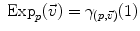 is called the exponential map at point
  . Straight lines going through 0 in the tangent space are transformed into geodesics going through point
  on the manifold and distances along these lines are conserved (Fig. 1).
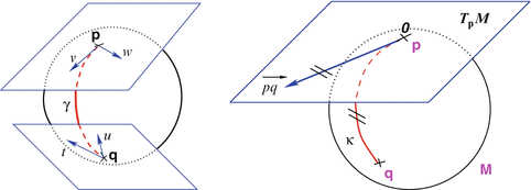
 are different: the vectors v and w of
  cannot be compared to the vectors
  and u of
  . Thus, it is natural to define the scalar product on each tangent plane. Right: The geodesics starting at
  are straight lines in the exponential map and the distance along them is conserved
 (since the manifold is geodesically complete) but it is generally one-to-one only locally around 0 in the tangent space (i.e. around
  in the manifold). In the sequel, we denote by
  the inverse of the exponential map: this is the smallest vector (in norm) such that
 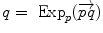 . If we look for the maximal definition domain, we find out that it is a star-shaped domain delimited by a continuous curve
  called the tangential cut-locus. The image of
  by the exponential map is the cut locus
  of point
  . This is (the closure of) the set of points where several minimizing geodesics starting from
  meet. On the sphere
  for instance, the cut locus of a point
  is its antipodal point and the tangential cut locus is the circle of radius
  .
. . It covers all the manifold except the cut locus of the reference point
  , which has a null measure. In this chart, geodesics starting from
  are straight lines, and the distance from the reference point are conserved. This chart is somehow the “most linear” chart of the manifold with respect to the reference point
  . The set of all the exponential charts at each point of the manifold realize an atlas which allows working very easily on the manifold, as we will see in the following.
2.3 Practical implementation
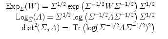
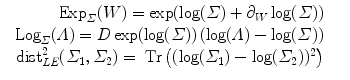
 and
and  is the basis of programming on Riemannian manifolds, as we will see in the following.
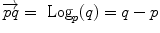 and
and 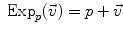 . This example is more than a simple coincidence. In fact, most of the usual operations using additions and subtractions may be reinterpreted in a Riemannian framework using the notion of bi-point, an antecedent of vector introduced during the 19th Century. Indeed, vectors are defined as equivalent classes of bi-points in a Euclidean space. This is possible because we have a canonical way (the translation) to compare what happens at two different points. In a Riemannian manifold, we can still compare things locally (by parallel transportation), but not any more globally. This means that each “vector” has to remember at which point of the manifold it is attached, which comes back to a bi-point.
 is as a vector of the tangent space at point
  . Such a vector may be identified to a point on the manifold using the exponential map
  . Conversely, the logarithmic map may be used to map almost any bi-point
  into a vector
  of
of  . This reinterpretation of addition and subtraction using logarithmic and exponential maps is very powerful to generalize algorithms working on vector spaces to algorithms on Riemannian manifolds, as illustrated in Table 1 and the in following sections.
Euclidean space | Riemannian manifold | |
|---|---|---|
Subtraction |  | 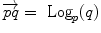 |
Addition |  |  |
Distance | 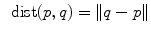 | 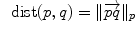 |
Mean value (implicit) | 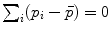 |  |
Gradient descent | 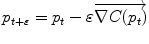 | 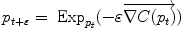 |
Geodesic interpolation |  | 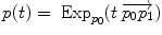 |
2.4 Example of Metrics on Covariance matrices
3 Statistical Computing on Manifolds
3.1 First statistical moment: the mean
 on the manifold that can be used to measure random events on the manifold and to define the probability density function (the function ρ such that
 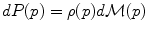 , if it exists). It is worth noticing that the induced measure
  represents the notion of uniformity according to the chosen Riemannian metric. This automatic derivation of the uniform measure from the metric gives a rather elegant solution to the Bertrand paradox for geometric probabilities [38, 62]. With the probability measure of a random element, we can integrate functions from the manifold to any vector space, thus defining the expected value of this function. However, we generally cannot integrate manifold-valued functions. Thus, one cannot define the mean or expected “value” of a random manifold element that way.
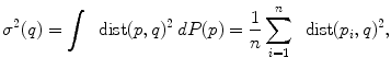
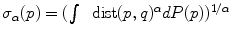 . The minimizers are called the central Karcher values at order α. For instance, the median is obtained for α = 1 and the modes for α = 0, exactly like in the vector case. It is worth noticing that the median and the modes are not unique in general in the vector space, and that even the mean may not exists (e.g. for heavy tailed distribution). In Riemannian manifolds, the existence and uniqueness of all central Karcher values is generally not ensured as they are obtained through a minimization procedure. However, for a finite number of discrete samples at a finite distance of each other, which is the practical case in statistics, a mean value always exists and it is unique as soon as the distribution is sufficiently peaked [37, 39].
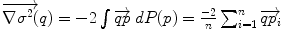 respectively in the continuous (probabilistic) and discrete (statistical) formulations. In practice, this gradient is well defined for all distributions that have a pdf since the cut locus has a null measure. For discrete samples, the gradient exists if there is no sample lying exactly on the cut-locus of the current test point. Thus, we end up with the implicit characterization of Karcher mean points as exponential barycenters which was presented in Table 1.
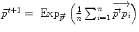 . One can actually show that its convergence is locally quadratic towards non degenerated critical points [22, 43, 55].
3.2 Covariance matrix and Principal Geodesic Analysis
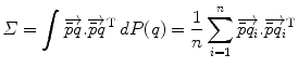
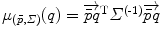 . Interestingly, the expected Mahalanobis distance of a random element is independent of the distribution and is equal to the dimension of the manifold, as in the vector case. This statistical distance can be used as a basis to generalize some statistical tests such as the mahalanobis D 2 test [57].
Related posts:

Stay updated, free articles. Join our Telegram channel

Full access? Get Clinical Tree


