Intracranial Arteries

The individual axial sections are usually supplemented with displays using MIP and, e.g., sagittal MPR as well as VRT (see above). A good diagnostic evaluation of the cerebral arteries can be achieved with thin overlapping section reconstructions using a section thickness of 0.6 to 1.25 mm and a reconstruction interval (RI) of 0.4 to 0.8 mm.

To achieve a high vascular contrast, the data acquisition has to be exactly timed to encompass the first passage of contrast medium through the circle of Willis with a start delay of 20 seconds, if possible before contrast medium has reached the venous sinus. If bolus tracking (BT) is not available, a test bolus should be injected to determine the individual circulation time. The following examination protocols can serve as guides for the visualization of the circle of Willis:

All scan protocols should be performed with automatic dose- and kV-modulation and with iterative recon with a mean strenght, if possible.

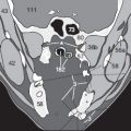
The subsequently reconstructed individual sections can display the vessels as seen from below with transverse MIP ( Fig. 178.1b ), from the front with coronal MIP ( Fig. 178.1c ) or from the side with sagittal MIP ( Fig. 179.1b ). The first two planes clearly show the major branches of the anterior (91a) and middle (91b) cerebral arteries.

Figure 178.1d shows a 3D VRT of another patient with an aneurysm () arising from the anterior communicating artery. The junction of both vertebral arteries (88) to form the basal artery (90) and posterior cerebral arteries (91c) is clearly identified. Furthermore, the branches of the anterior circulation are identifiable: branches of the medial cerebral artery (91b) and the pericallosal arteries (93).

Venous Sinus

To visualize the venous channels, the FOV has to be extended to the sagittal cranial vault ( Fig. 179.1a ) and the start delay increased to about 100 seconds. Craniocaudal sections are recommended for both types of CTA (arterial and venous cerebral vessels). The sagittal plane ( Fig. 179.1b ) preferably shows contrast in the vein of Galen (100) and venous channels (101a, 102a).

Venous Sinus Thrombosis

In cases of normal venous flow in the cerebral sinuses, you will find hyperdens lumina of both transverse sinuses ( in Fig. 179.2a ) as well as both sigmoid sinuses ( in Fig. 179.2b ) without any filling defects in contrast-enhanced images.

In contrast to this, Fig. 179.3 shows unilateral thombosis of the left sigmoid sinus () and bilateral thrombosis of both transverse sinuses ( ).

3D-reconstructions and MIPs might be time-consuming to create, because of the adjacent hyperdense skull, which has to be eliminated first by the investigator at the workstation, before the reconstructions can be done – and they often do not provide useful additional information.

„Triple-Rule Out“ protocol

On pages 182–186, you will find special protocols to look for aortic aneurysm, coronary artery stenosis or calcifications and for pulmonary emboli. This protocol might be used to clarify all three issues with only one spiral scanning.

Carotid Arteries

Important criteria for stenotic processes of the carotid arteries are the exact determination of the severity of the stenosis. It is for this reason that the examination is carried out with thin sections, for instance, 4 x 1 mm or 16 x 0.75 mm, allowing direct planimetric quantification of the stenosis with adequate accuracy on individual axial sections. Furthermore, the sagittal and coronal MIP (0.7 – 1.0 mm RI with 50% sectional overlapping) shows no major step deformity (see page 8).

The best reconstruction with maximal contrast of the carotid artery is achieved with minimal contrast in the jugular vein. Therefore, the use of a bolus tracking program is strongly advised. If a preceding Doppler examination suggests a vascular process at the bifurcation, transverse images in caudocranial direction are recommended. For processes near the cranial base, a craniocaudal direction can be superior. VRT often proves helpful to get oriented ( Figs. 180.1d, 180.2b ).

Figure 180.1 shows the lateral topogram (a) for positioning of the FOV as well as lateral (b) and anterior (c) images of an MIP and an image in VRT (d), showing normal findings. In contrast, Figure 180.2 shows images of sagittal MIP and VTR that reveal two indentations of the vascular contrast column at the typical site for a carotid stenosis: The left ACI (85a) shows a short segment of a severe luminal narrowing just distal to the bifurcation () after a preceding bulbar stenosis () of the ACC (85) at the origin of the ACE (85b).

Aorta

The CT angiography of the aorta must above all exclude aneurysms, isthmus stenoses and possible dissection, and if present, visualize their extent. Automatic bolus tracking (BT: ROI placed over the aorta) is advisable, especially in patients with cardiac diseases who have variable pulmonary circulation times of contrast medium. Imaging in caudocranial direction can minimize the respiration-induced motion artifacts that primarily affect the regions close to the diaphragm since involuntary respiratory excursions are more likely at the end of the examination. Furthermore, caudocranial imaging avoids the initial venous inflow of contrast medium through the subclavian and brachiocephalic veins and any superimposition on the supra-aortic arteries.

As reconstruction images, MIP and MPR ( Figs. 182.3, 182.4 ) often allow an exact quantification of the vascular pathology as survey images in VRT ( Fig. 182.5 ), as seen here as an example of an infrarenal aneurysm of the abdominal aorta: The aneurysmal dilatation (171) begins immediately distal to the renal arteries (110) and spares both the superior mesenteric artery (106) and iliac arteries (113).

For planning any vascular surgery, it is crucial to know any involvement of visceral and peripheral arteries and any possible associated dissection. Furthermore, the level of the aortic origin of the artery of Adamkiewicz, which supplies the thoracospinal transition of the spinal cord, must be considered a b for aneurysms of the descending thoracic aorta.

Frequently, a cine mode review of the coronal or sagittal MPR images on a second monitor can be helpful for a quick and convincing determination of the extent of a pathologic finding, as shown here in a case of thrombosis within an abdominal aortic aneurysm. The cine mode of the coronal MPR images reveals not only an infrarenal thrombus (173) along the left lateral wall ( Fig. 183.1 ) but also a second thrombus further cranial along the right lateral wall at the level of the origin of the right renal artery (110) ( Fig. 183.1 ), which is still perfused ( Fig. 183.3 ). The individual axial sections ( Figs. 183.4, 5 ) allow a planimetric quantification of the stenosis, and the sagittal MPR ( Fig. 183.6 ) a clear separation from the origin of the anterior mesenteric artery (106).

Of course, the benefit of the three-dimensional visualization by means of VRT also depends on the viewing angle. While viewing from an angle ( Fig 183.7 ) can underestimate the extent of the thrombus and easily mistake it for a soft plaque, the extent is much better appreciated if seen from different viewing angles ( Figs. 183.8 and 183.9 ). The final images illustrate the effect of a careful elimination of interfering superimposed osseous structures. Because of its high density, the lumbar spine dominates the initial image ( Fig. 183.8 ), and the vascular findings are only fully appreciated after subtraction of the lumbar spine ( Fig. 183.9 ).