CT Image Reconstruction Basics
Joachim Hornegger
Andreas Maier
Markus Kowarschik
Computed tomography perfusion (CTP) imaging requires the reconstruction of a series of time-dependent volumetric datasets. The sequence of CT volumes measures the dynamics of contrast agent both in the vasculature and in the parenchyma.
CT image reconstruction refers to the computational process of determining tomographic images from x-ray projection images of the irradiated patient. Image reconstruction is a computationally intensive task and one of the most crucial steps in the CT imaging process.
As the basics of x-ray physics were detailed in Chapter 1, the reader should assume that the result of the x-ray image formation is an attenuation image. Each individual pixel on the detector, therefore, represents a line integral, that is, the accumulation of all x-ray attenuation coefficients along the projection line. Here, the projection line is the connecting line of the x-ray focal spot with the center of the respective detector pixel.
From Line Integrals to Voxels
Despite the discrete nature of the projection images, most reconstruction theory uses a continuous framework, in which the reconstruction algorithms are derived mathematically. The problem of discrete sampling is then solved within the final formulation of the reconstruction algorithm. As the discrete sampling is a more technical issue, it is neglected here for the ease of presentation, and the reader should refer to the literature that details these steps.1 Thus, the description will remain in a continuous domain in this section.
Radon Transform
For ease of understanding, this approach is explained in the two-dimensional (2D) (x, y) plane. The source-detector arrangement is rotating around the object (Fig. 2.1). In the following, Dirac’s δ-function is used to select the parts of the object that are traversed by the x-ray. Recall that δ(t) is zero everywhere except at t = 0, where δ becomes infinite. Furthermore, the δ-function fulfills for any real-valued function g(x) the shifting property:
A parallel projection p(s, θ) at detector element s and at source/detector array rotation angle θ can be written in the following notation:
where f (x, y) represents the x-ray attenuation coefficient at object location (x, y). Thus, the δ-function selects the line x cos θ + y sin θ = s that connects the detector and the source array at s while both arrays are rotated by θ. Thus, p(s, θ) describes a line integral whose value is observed at the detector.
This process of turning function values f (x, y) into line integral values p(s, θ) is also referred to as the Radon transform in 2D. The fundamental problem of CT reconstruction is the computation of function values f(x, y) from the measured line integral values p(s, θ); that is, the inverse Radon transform.
Another important concept in CT reconstruction is back-projection, as described in the following. Backprojection is a kind of conjugate (but not inverse) process to the (forward) projection. For the case of parallel-beam x-ray projections, it assigns to a point (x, y) in object coordinates the integral b(x, y) of the projection values that lie on the x-rays passing through (x, y):
Fourier Slice Theorem
The Fourier slice theorem is fundamental to many CT reconstruction approaches. It states that the 1D Fourier transform P(ω, θ) of a projection p(s, θ) in parallel-beam geometry for a fixed rotation angle θ is identical to the 1D profile through the origin of the 2D Fourier transform F (ω cos θ, ω sin θ) of the irradiated object (x, y). Figure 2.2 displays this process.
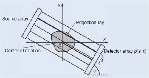 FIGURE 2.1. Parallel-beam geometry and the generation of a parallel-beam projection p (s, θ). |
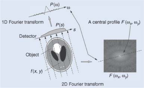 FIGURE 2.2. Illustration of the Fourier slice theorem. |
Filtered Back-Projection for 2D Parallel-Beam Geometry
With the Fourier slice theorem one of the most commonly used reconstruction algorithms—the filtered back-projection (FBP) method—can be elegantly derived. A derivation is shown in the Geek Box, Fourier slice theorem Proof. The resulting algorithm uses two concepts: (i) filtering and (ii) back-projection.
The filter h(s) is called ramp filter because of the shape of |ω|. This filter corrects the oversampling that occurs at the center of the Fourier space. This is accomplished by enhancing high spatial frequency components while dampening low spatial frequency components. In practice, this filtering operation is often combined with additional filtering to achieve certain image characteristics. Various kernels can be created and embedded into the reconstruction process to obtain smoother or sharper images.
Geek Box: Fourier Slice Theorem Proof
To prove this, we start with the 1D Fourier transform P(ω, θ) of p(s, θ):
Using the definition of the projection p(s, θ), we obtain
Rearranging the order of the integrals then yields
which, after elimination of the delta function, reads as
Finally, using the definition of the 2D Fourier transform, we obtain
which results in the proposed statement
By varying θ, we get the complete Fourier transform Fpolar(ω, θ) of the unknown function f(x, y) in polar coordinates (ω, θ).
Geek Box: Derivation of the Filtered Back-Projection Algorithm
To illustrate this derivation, we start with the inverse Fourier transform F(u, v):
and rewrite it to polar coordinates Fpolar(ω, θ):34
According to the Fourier slice theorem, we obtain
which contains a product of the projection in 1D Fourier space P(ω, θ) and |ω|. The inverse Fourier transform of P(ω, θ). |ω| corresponds to a convolution in spatial domain. The inverse Fourier transform of |ω| shall be defined by the filter kernel h(s). Hence, in spatial domain, the previous equation can then be written as
which is the back-projection of the projection data p(s, θ) convolved with h(s).
After filtering, the projection data is back-projected into image space, as described in the previous section. Note that the FBP algorithm uses the Fourier slice theorem only implicitly. That is, both filtering and backprojection can be implemented in a way that the actual computation of the Fourier transform is not required. However, as the ramp filter is a global operation, the implementation using fast Fourier methods is often favorable.
Acquisition Geometries
The filtered back-projection algorithm is an efficient and robust method for the computation of tomographic slice images. Using a fan-beam geometry based on a single x-ray source that is collimated toward a curved array of detector elements, it is possible to circumvent long acquisition times and bulky hardware that would be required for parallel-beam geometry. Doing so, a single source is sufficient to collect multiple rays at the same time (see Fig. 2.3), but the Fourier slice theorem cannot be applied straightforwardly.
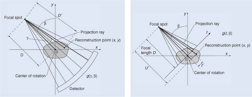 FIGURE 2.3. With fan-beam geometry, one is able to image multiple detector elements at the same time with only one x-ray source. Depending on the type of detector, two different geometries emerge. Using a curved detector, an equiangular geometry described by g (γ, β) is obtained (left), and using a linear detector, an equally spaced geometry denoted by g (t, β) is created (right). |
If a full rotation with either parallel-beam or fan-beam acquisition geometries is performed, one can easily observe that both geometries cover identical data. They are merely collected in a different sequence. If β is considered as the rotation angle of source and detector, γ as the angle to the respective detector elements, and D as the source-to-rotation axis distance, the following relations between identical rays in fan-beam and parallel-beam geometry are obtained:
This relation offers two possible solutions for image reconstruction. Either the projection data is reordered into parallel-beam geometry in a so-called “rebinning” step, or the reconstruction algorithm has to be adapted to the acquisition geometry. Both algorithms are used in practice. The interpolation operation in the rebinning step must be handled with caution as it may lead to an unintended loss in image resolution. The Geek Box, Fan-Beam Reconstruction without Rebinning, sketches an idea how to obtain an algorithm without rebinning.
Geek Box: Fan-Beam Reconstruction without Rebinning
To omit rebinning, one has to reshape the filtered back-projection reconstruction formula by a change of coordinates of the integral variables s and θ according to the ray identities in Eq. (rays). This yields the following fan-beam reconstruction formula for a curved detector:

Note that we introduced the variables D′ = D′(x, y, β) and γ′ = γ′(x, y, β) that describe distance and angle of the reconstructed point (x, y), as shown in Figure 2. This equation can be interpreted as a convolution of the fan-beam projection g(γ, β) with a fan-beam ramp filter
 . Furthermore, a weighting factor cos γ is applied. This weighting is also referred to as the cosine weight.1
In case of a linear detector with equally spaced detector elements, a slightly different reconstruction formula is obtained, as the integral variables are substituted to t and β, where t is the index of the detector element:
Again, we introduced several variables: the index t′ = t′(x, y, β) of the projection of the reconstruction point (x, y) on the detector and the depth U′ = U′(x, y, β), as shown in Figure 2.2. In this formulation, we find the parallel-beam ramp filter h(t′ – t) from the previous section. It is applied to a fan-beam projection g(t, β). Prior to the convolution, this projection was weighted with the factor
 , the cosine-weight for the linear detector case. Note that the back-projection is weighted with a distance weight (U′)−2, which is dependent on the image point to be reconstructed.
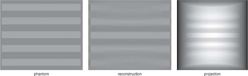 FIGURE 2.4. Effect of the cone-beam geometry in a circular trajectory with a cone angle of 30 degrees. From left to right: XZ slice of the original Defrise disk phantom,2 the XZ slice of the reconstructed volume using the FDK algorithm, and the projection image for all projection angles. |
Modern CT scanners introduced multirow detector arrays. These arrays introduce a second dimension on the detector and the rays from source to detector form a cone. This cone-beam geometry allows even faster data acquisition. However, the acquisition geometry has to be decided with care, as the rays do no longer fall into the same plane. Hence, even if rotation is performed on a full circle, there are rays that are required for reconstruction that are not collected. This missing data causes artifacts in the reconstruction result that are called cone-beam artifacts (Fig. 2.4).
In a divergent beam scenario, only those line integrals that intersect the path of the x-ray source can be measured as all x-rays originate from there. This path is also referred to as the source trajectory. To create a theoretically correct reconstruction result, a complete data set must be acquired. According to Tuy’s sufficiency condition,2 every plane that intersects the object has to intersect the path of the x-ray source. Figure 2.5 shows examples of incomplete and complete trajectories. Although a circular trajectory is insufficient, as planes that are parallel to the plane of rotation do not intersect with the source trajectory, this problem can be resolved by adding lines to it (see Fig. 2.5, bottom left). A more elegant way is to rotate the source along a helical path as a continuous motion is obtained. Note that a change in the path of the trajectory also often implies a different reconstruction algorithm. For tilted gantries and helical trajectories, for example, the reconstruction method, the size of the field of view, and the length of the pitch have to be adjusted. If the standard reconstruction method is not adjusted in an appropriate manner, it will cause in severe artifacts in the reconstructed image.3
Related posts:
 Clinical Applications and Theoretical Principles: Primer on Physics of MR and Hardware
 Flow Territory Mapping: Region-Selective Arterial Spin Labeling
 Cerebrovascular Anatomy and Regional Blood Supply
 Tumor Vasculature: Structure and Function
 Gastrointestinal Imaging
 Cerebral Perfusion Studies in Substance Abuse and Dependence
Stay updated, free articles. Join our Telegram channel

Full access? Get Clinical Tree


