Data Analysis and Image Processing
Robert Koeppe
The goal of positron emission tomography (PET) is to make use of tracers labeled with positron-emitting radionuclides for the purposes of diagnostic imaging. PET, a nuclear medicine imaging procedure, differs from standard radiological x-ray procedures in that the radiation detected by the imaging device originates and is emitted from within the subject’s body rather than originating from an external source and being transmitted through the body. PET studies, like all nuclear medicine radioisotope emission procedures, yield images that represent the distribution of the radiotracer within the body. This distribution or pattern of uptake and incorporation depends on the physiologic, pharmacologic, and/or biochemical state of the individual’s body. In contrast, images produced by conventional x-ray procedures reflect x-ray attenuation and are governed by the physical composition of the body. Thus, nuclear medicine procedures in general and PET procedures in particular are capable of providing information concerning how the body is functioning at a physiologic or biochemical level, while x-ray procedures such as computed tomography (CT) primarily depict human anatomy. Although PET does provide limited anatomic information and some functional information can be derived from CT, each technique is useful in its own way. As we will see later in this and other chapters, recent advances in both hardware and software allow the combination of functional and anatomic information, improving both the ability to answer scientific questions and the overall diagnostic utility of tomographic imaging methods.
PET procedures have the additional potential for providing quantitative measures of radiotracer concentration in a living biological system at spatial resolutions of a few millimeters and with subminute temporal resolution. Methods for obtaining quantitative images of radiotracer concentration from PET involve a technique called image reconstruction from projections. For many PET applications, these quantitative measures of radiotracer concentration can be extended to yield more pertinent measures of biological function through the use of compartmental analysis and tracer kinetic modeling. Analysis of a temporal sequence of radiotracer images allows estimates of parameters representing specific physiologic processes such as blood flow, glucose metabolism, protein synthesis, neurotransmitter or enzyme levels, and receptor or binding site density. The production of different positron-emitting radionuclides and the synthesis of a variety of PET radiopharmaceuticals described in Chapters 1 and 2 allow one to study many distinct aspects of organ systems within the functioning human body.
The purpose of this chapter is to discuss the basic principles involved in the production and processing of PET images and to describe various methods used to analyze the quantitative data produced by PET. The goal of image reconstruction and its associated steps is to produce the most accurate images of radiotracer concentration possible, with the highest signal-to-noise (SNR) and at the highest spatial resolution. The primary goal of compartmental modeling is to provide more valuable information related to the functional state of the subject than can be provided by images of radioactivity distribution alone. The overall goal of image display techniques is to provide both spatial and functional information in a visually optimal manner. The following sections describe the theoretical concepts of and methods for (a) image reconstruction from projections, including the additional steps and corrections specific to PET data; (b) compartmental modeling, including data acquisition requirements, curve fitting, parameter estimation, and model validation; and (c) methods for combining and displaying both functional and/or anatomic information for multiple imaging studies (although this is expanded upon in a subsequent chapter).
Image Reconstruction from Projections
In conventional nuclear medicine gamma camera imaging or in simple x-ray imaging, information from the three dimensions of a
human subject gets collapsed onto a two-dimensional (2D) image. There is ambiguity in such images as all information from one dimension is represented by a single point or pixel of the 2D image. For gamma camera images, radioactivity from different locations within the body appears overlaid upon itself. Tomography, or slice imaging, is a method that allows a three-dimensional (3D) object to be depicted as a series or stack of thin 2D cross-sectional images. Each image of the series represents only two dimensions of object, while information on the third dimension is contained in the different images of the series. Although this appears simple in concept, imaging devices have the inherent problem of recording information from three dimensions on 2D detector surfaces. Thus, each acquired data point recorded still represents information integrated along one dimension of the object. These integrals or weighted sums are referred to as projections or projection rays. Image reconstruction from projections is the mathematical technique or groups of techniques that allow the construction of the set of cross-sectional images, each representing only two dimensions of information.
human subject gets collapsed onto a two-dimensional (2D) image. There is ambiguity in such images as all information from one dimension is represented by a single point or pixel of the 2D image. For gamma camera images, radioactivity from different locations within the body appears overlaid upon itself. Tomography, or slice imaging, is a method that allows a three-dimensional (3D) object to be depicted as a series or stack of thin 2D cross-sectional images. Each image of the series represents only two dimensions of object, while information on the third dimension is contained in the different images of the series. Although this appears simple in concept, imaging devices have the inherent problem of recording information from three dimensions on 2D detector surfaces. Thus, each acquired data point recorded still represents information integrated along one dimension of the object. These integrals or weighted sums are referred to as projections or projection rays. Image reconstruction from projections is the mathematical technique or groups of techniques that allow the construction of the set of cross-sectional images, each representing only two dimensions of information.
Historical Background
The beginnings of image reconstruction from projections occurred with a 1917 paper published by the Austrian mathematician J. Radon (1). In this work, he proved that a 2D or 3D object can be reconstructed exactly from the full set of its projections, a projection again representing the object integrated along one dimension. It was not until the 1950s to 1970s when this result was rediscovered by people in several different fields including mathematics (2,3), radio astronomy (4), and electron microscopy (5), in addition to medical imaging (6,7,8), that applications for image reconstruction from projections began to be found. Although the first suggestions of using positron-emitting radionuclides for medical imaging arose in the 1950s (9,10,11,12) and the first positron tomographic imaging devices appeared in the 1960s (13) and 1970s (14), the practical application of PET imaging followed that of single-photon emission computed tomography (15,16) (SPECT) and did not occur until the mid- to late 1970s.
As the field exploded throughout the 1970s, hundreds of papers relating to image reconstruction from projections were published in prominent journals from the fields of mathematics, physics, engineering, and biomedicine. Several reviews of reconstruction algorithms were written (17,18,19) summarizing the few different general approaches and the many different specific implementations of image reconstruction algorithms.
Reconstruction Algorithms
Although reconstruction algorithms can be categorized in several different ways, most algorithms for PET can be classified into two general approaches: reconstruction by filtered back projection and iterative reconstruction. Before discussing these approaches we will review some concepts common to both.
Projection Data
As described in Chapter 3, the data acquired directly by the PET scanner represents the sum or integral of radioactivity along the lines connecting any given pair of detectors, often referred to as lines of response (LOR). This is true for both 2D and 3D data acquisition. The following paragraphs describe the basics of 2D-image reconstruction, most of which applies to 3D reconstruction as well. Specific issues related to 3D-image reconstruction will be discussed in the section “Image Reconstruction for Three-Dimensional PET.”
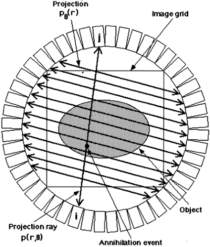 Figure 5.1. Projection data for two-dimensional PET acquisition. The diagram represents a single detector ring containing 48 detectors. A coincidence line of response between a given pair of detectors i and j is called a projection ray, p(r,θ), and can be defined in terms of an angle 0 and the distance r that the line passes from the center of the field of view. The projection ray data give the sum or integral of radioactivity along the line connecting the two detectors. A set of all projection rays having the same angle θ is referred to as a projection and is denoted by pθ(r). Each projection Pθ represents one complete view of the object. |
Assume the true 2D radiotracer distribution that we are imaging is given by the function f(x, y), where x and y are standard Cartesian coordinates. The measured PET data, as depicted in Fig. 5.1, can be represented by:
where (x′, y′) are the coordinates in a Cartesian system rotated by the angle θ.
Each (x′, θ) pair of the projection data represents a single line integral that in turn corresponds to a specific pair of detectors (line of response). A given p(x′, θ) often is called a projection ray. The collection of projection rays with the same angle θ is referred to as a projection. Thus, we also can define pθ(x′) as an equivalent representation of
the projection data, but one used when referring to the collection of projection rays as a whole rather than the individual rays, p(x′, θ). All the rays of a given projection pθ(x′) are parallel, where x′ is a simple linear measure of the position of each ray within the projection. It is important to note that each projection pθ of the 2D object has only one dimension. Thus, the 2D projection data defined by p(x′, θ) can also be thought of as a set of one-dimensional projections, pθ(x′). Each individual member of this set of projections is defined by a single angle (θ) and represents one complete view of the object. By a complete view, it is meant that each point of the object f(x, y) is included in one and only one ray of each projection. Thus, in a perfect noise-free system, the sum over all rays of a given projection is the same for all projections and is proportional to the total radioactivity in the object:
the projection data, but one used when referring to the collection of projection rays as a whole rather than the individual rays, p(x′, θ). All the rays of a given projection pθ(x′) are parallel, where x′ is a simple linear measure of the position of each ray within the projection. It is important to note that each projection pθ of the 2D object has only one dimension. Thus, the 2D projection data defined by p(x′, θ) can also be thought of as a set of one-dimensional projections, pθ(x′). Each individual member of this set of projections is defined by a single angle (θ) and represents one complete view of the object. By a complete view, it is meant that each point of the object f(x, y) is included in one and only one ray of each projection. Thus, in a perfect noise-free system, the sum over all rays of a given projection is the same for all projections and is proportional to the total radioactivity in the object:
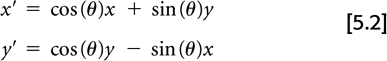
The entire collection of projection data when plotted as θ versus x′ is called a sinogram since a point source in the object traces a sinusoidal pattern, as shown in Fig. 5.2. It is not mandatory to group the projection rays into parallel collections, as described here, but one can choose other groupings such as all rays that contain a common detector. For 2D data, this particular grouping of projection rays would create a fan-shaped projection, and thus is referred to as fan-beam geometry (x-ray CT terminology). Note though that a single projection still consists of a complete view of the object. Specific groupings may be beneficial for specific applications, however, throughout this chapter the parallel-ray geometry will be retained.
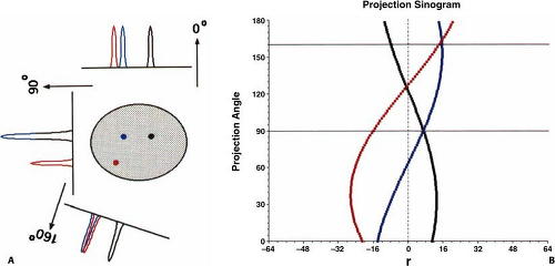 Figure 5.2. Two-dimensional projections and projection sinogram. A: The top of the illustration depicts an elliptical two-dimensional object containing three discrete points of equal radioactivity (red, blue, and black dots). A full set of projections covers angles from 0 degrees to 180 degrees. Three sample projections are shown at 0 degrees, 90 degrees, and 160 degrees. Due to the finite resolution of a PET system, point sources appear within a projection roughly as Gaussian distributions (red, blue, and black curves). If the points fall along different rays within a projection as in p0°, the resultant curves in the projection are of equal magnitude and are separated spatially. If two of the points fall along the same ray, as seen in p90°, only two curves are seen, the red curve representing radioactivity from one point, and the blue/black curve having twice the magnitude, representing radioactivity from the other two points. The 160-degree projection shows a case where two of the points are slightly offset. The resolution of the PET system determines how large a difference in r or θ is necessary to distinguish between two points within an object. Part B shows the projection sinogram for this object. A sinogram is a plot of all the projection rays p(r, θ), sorted as projection angle θ versus r. Note that each point of the object traces out a sinusoidal pattern in this plot, hence the name sinogram. Compare the three projections in A with the three horizontal lines in B corresponding to projection angles at 0 degrees, 90 degrees, and 160 degrees. Note that the blue and black traces intersect at 90 degrees, while the red and blue traces nearly overlap at 160 degrees. |
Filtered Back-Projection
One method of reconstructing images from their projections is called filtered back-projection (FBP). As the name implies, this involves two principal steps: filtering the projections and then back-projecting them to create the reconstructed image. The operation of back-projection in terms of the projection data, p(x′, θ), from our 2D object, f(x, y), is given by:
Back-projection in one sense is the converse operation to the forward-projection that occurs naturally during PET data acquisition. That is, the act of PET data acquisition itself transforms a 2D array of values into sets of projections or line integrals, while back-projection converts the projection set back to a 2D array. Note, however, that forward-projection followed by simple back-projection does not yield the original object. As shown in Fig. 5.3, an object consisting of a single point source is represented by projection data having a single nonzero value at each projection angle. As these data are back-projected, each angle θ creates a line in the reconstructed image. Thus, a point source object yields an image with a starlike pattern. To arrive back at the true object, the projection data must be modified or filtered prior to back-projection.
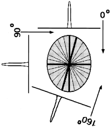 Figure 5.3. Two-dimensional back-projection. Depicted is an object containing a single point of radioactivity located at the center of the field of view. Each projection contains a single peak representing the radioactivity from this point. Back-projection (without filtering) consists of taking the data from each projection and “smearing” them back along the rays of the projection. Note that the arrows are shown in the opposite direction, representing the operation of back-projection, than those of Fig. 5.2 that represent the inherent forward-projection operation of data acquisition. The dark lines correspond to the back-projections along three angles—0, 90, and 160 degrees. The lighter lines correspond to back-projections along other projection angles. The resultant back-projected image, however, is not a single point, but a starlike pattern centered on the location of the point. This result demonstrates why “filtering” the projections is necessary before the back-projection step. |
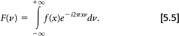
Before describing the filtering step, the concept of the Fourier transform must be introduced. A one-dimensional Fourier transform of a one-dimensional function f(x) is a frequency space representation of f(x). By this we mean that any function f(x) can be described as the sum of sin or cos functions having varying frequencies and magnitudes, F(ν). The value of F(ν) gives the magnitude of the sinusoidal function with frequency ν. The Fourier transform is defined mathematically as:
The Fourier transform of F(ν) yields the original function f(x). This transform from F(ν) back to f(x) is called an inverse Fourier transform, although the mathematical formulas for both transforms are identical.
From Radon’s work, it can be shown that if the Fourier transform of the projection data at angle θ:
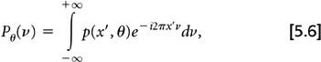
is multiplied by ν,
then the inverse Fourier transform of PθF
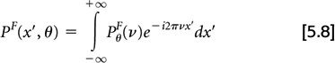
yields a filtered projection, pF(x′,θ), which under noise-free conditions yields the true object when back-projected:
The frequency-space filter, ν, is commonly known as a “ramp” filter. To summarize, image reconstruction by FBP consists of four steps applied to each projection θ from 0 to 2π: (a) Fourier transform the projection, (b) filter the transformed projection in frequency space, (c) inverse Fourier transform the filtered frequency space projection, and (d) back-project the filtered projection.
A major limitation of PET image reconstruction using filtered back-projection is statistical noise. The distribution of spatial frequencies (the power spectrum) of the actual (i.e., noise-free) radiotracer distribution tends to decline at higher frequencies, while statistical noise tends to have a fairly uniform frequency distribution, close to “white” noise. The multiplication in frequency space by a ramp filter amplifies the higher frequencies that tend to be dominated by noise, thus causing decreased SNR in the reconstructed images. To control noise, a postreconstruction smoothing filter can be applied, or more commonly, the ramp filter is modified to preferentially reduce higher frequencies in the projection data. Although many different filter functions have been employed (Butterworth, Hamming, Parzen), all have the same general property that they “roll off” at higher frequencies as shown in Fig. 5.4. Although filters that have a sharper roll off suppress more noise, they also reduce high-frequency signal, thus creating an inherent tradeoff between noise and spatial resolution. In practice, projection data are not continuous but discrete. Shannon’s sampling theorem states that the maximum frequency that can be represented by the data, called the Nyquist frequency (νN), equals 1 divided by twice the sampling frequency, νN = 1/(2x′). Trying to recover higher frequencies produces errors in the reconstruction images called aliasing artifacts. Thus, the frequency space filter extends from 0 to the Nyquist frequency.
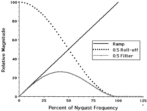 Figure 5.4. Back-projection filters. For noise-free data, a linearly increasing “ramp” function in Fourier space gives the appropriate filter necessary for exact reconstruction of the object. The noise in PET data, however, has a fairly uniform frequency distribution; thus, a ramp filter amplifies the high-frequency noise and results in noisy-looking images. To limit noise propagation, the ramp filter is rolled off at higher frequencies. The roll-off function (shown for a Hamming 0.5 filter) is multiplied by the ramp filter to yield the final filter function. |
Fourier transforms, while useful, are not essential for FBP. This is because of an equivalence between the convolution of two functions and the product of their Fourier transforms.
By applying this principle to Equations 5.7 and 5.8, the filtered projection, pF(x′, θ), can be obtained by taking the inverse Fourier transform of the frequency space filter W(ν) and convolving it with the raw projection data p(x′, θ):
and thus
where F–1 represents the inverse Fourier transform.
The noise properties of filtered back-projection for low count studies, such as occur in many whole-body fluorine-18-fluorodeoxyglucose ([18F]-FDG) scans, plus the additional noise and significant artifacts associated with transmission scanning and patient movement (see the section “Attenuation” below) have prompted much effort in the development alternative algorithms for image reconstruction. The vast majority of these techniques fall into the category of iterative reconstruction techniques.
Iterative Reconstruction
Iterative reconstruction techniques are not a recent development, but have been available and used for PET as long as filtered back-projection. The main limitation in the past has been the greater computational requirements for iterative methods than for FBP. This section outlines the basic steps of iterative reconstruction. The following section describes advances that have made iterative techniques readily available for routine use.
Rather than using an analytic solution to produce an image from the projection data, iterative reconstruction makes a series of estimates of the image, compares forward-projections of these estimates to the measured data, and refines the estimates by optimizing an objective function until a satisfactory result is obtained. Iterative methods have several advantages over FBP. They allow more accurate modeling of the data acquisition system than the line-integral model used by FBP and more accurate modeling of the statistical noise in emission and transmission images. An additional advantage is that iterative methods can incorporate a priori information about the object being scanned into the reconstruction process. For example, since radiotracer concentration is being imaged, all image values must be greater than or equal to zero. Thus, a nonnegativity constraint can be included in the optimization. Another use of a priori information is the incorporation of anatomic boundaries from coregistered CT or magnetic resonance (MR) scans with a constraint designed to allow differences across boundaries but penalize differences within boundaries.
The three key steps of an iterative algorithm are: (a) determination of a model describing the data acquisition system (including noise), (b) a calculation using the objective function that quantifies how well the image estimate matches the measured data, and (c) an algorithm that determines the next estimate of the image. The model for the measured data takes the general form p = Af, where p = {pj, j = 1, …, m} is a vector containing all m values of the measured projection ray data (i.e., p(x′, θ) for all (x′, θ) pairs), f = {fi, i = 1, …, n} is a vector containing the values of all image voxels (i.e., f(x, y) for all (x, y) pairs), and A = {Aij} is a forward-projection matrix for mapping f into p. Matrix A is often called the system, design, or transition matrix. The elements of the matrix Aij contain the probabilities of a positron annihilation event occurring in voxel
i being detected in projection ray j. Several additional unwanted processes, such as random and scattered coincidences, which will be discussed below, affect the measured projection data, thus complicating the general model. These can be incorporated into a system model of the form p = Af + r + s, where r and s are vectors representing the random and scattered events included in the measured projection data p, although a discussion of more complex system models is beyond the scope of this chapter. The objective function includes any a priori constraints such as nonnegativity and smoothness. Typical objective functions include the Poisson likelihood and the chi-square error (the Gaussian likelihood). The iterative algorithm must ensure that successive estimates of the image converge toward a solution that maximizes (or minimizes) the objective function. The algorithm must also have an exiting criterion that defines when to terminate the iteration process.
i being detected in projection ray j. Several additional unwanted processes, such as random and scattered coincidences, which will be discussed below, affect the measured projection data, thus complicating the general model. These can be incorporated into a system model of the form p = Af + r + s, where r and s are vectors representing the random and scattered events included in the measured projection data p, although a discussion of more complex system models is beyond the scope of this chapter. The objective function includes any a priori constraints such as nonnegativity and smoothness. Typical objective functions include the Poisson likelihood and the chi-square error (the Gaussian likelihood). The iterative algorithm must ensure that successive estimates of the image converge toward a solution that maximizes (or minimizes) the objective function. The algorithm must also have an exiting criterion that defines when to terminate the iteration process.
The most extensively studied iterative algorithm is the maximum-likelihood expectation-maximization (MLEM) (20), which seeks to maximize the logarithm of the Poisson likelihood:
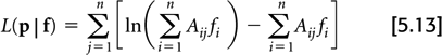
In practice, the logarithm of the likelihood function is maximized instead of the likelihood function itself for computation reasons, and since they both are maximized for the same image, f.
The EM algorithm updates the voxel values (fi) by:
where fk and fk+1 are the image estimates from iteration k and k + 1, respectively. Note the double summations over i and j. It is these steps that make the algorithm computationally demanding.
Reduction in Computational Load
As mentioned earlier, the main limitation of iterative reconstruction is its high computational load. For many algorithms, one iteration requires about twice the time of FBP. Thus, considerable effort has been directed not only toward maximizing algorithm performance with respect to image quality, but also toward the development of schemes that converge rapidly. If sufficient quality image estimates can be obtained in 5 instead of 50 iterations, the computation time of iterative routines might well be acceptable.
A significant breakthrough in iterative reconstruction speed occurred with the introduction of reconstruction using ordered subsets (OS) of projection data (21). The concept of ordered subsets can be applied to any iterative algorithm; however, the initial paper and the majority of implementations have paired OS with the EM algorithm, thus yielding the common acronym OSEM. For OSEM, the projection data are grouped into subsets. A standard EM algorithm is then applied to one of the subsets using the appropriate rows of the system matrix. The resulting reconstruction becomes the starting value to be used with the next subset. A single iteration of OSEM is completed when each of the subsets has been used once. Assuming mutually exclusive and exhaustive subsets (i.e., each projection ray is a member of one and only one subset), a single OSEM iteration requires approximately the same computation time as one standard EM iteration. However, “convergence” is much faster. Further iterations can be performed by making additional passes through the same “ordered” subsets. Results from Hudson and Larkin’s study show that one or two iterations with either 32 or 16 subsets yield images with lower chi-square and mean-square error than images with 20 or 30 iterations with standard EM (21). Reconstructed images appear visually similar as well. In general, to achieve a reconstruction with a given error level, the number of iterations required is inversely proportional to the number of subsets used.
For implementation with PET, each subset may include several projection angles (a projection being the complete set of parallel projection rays at one angle). The order that the projections are processed is arbitrary from the standpoint of the algorithm; however, particular orders improve image quality and accelerate convergence. For example, selecting projections that are widely and evenly spaced, hence containing substantially different information, is better than selecting projections that are close in angle and do not vary considerably from one another. For the detector configuration of the ECAT Exact scanner, (CTI, Inc., Knoxville, TN) a single 2D sinogram consists of 192 projections, 168 rays per projection. A 32-subset implementation of OSEM uses only six projections per subset (192 projections per 32), with 30 degrees between each projection of the subset.
A problem with the OSEM algorithm is that, except for noise-free data, the solution does not converge to the maximum likelihood solution. Other rapid statistical algorithms, including row-action maximum-likelihood and space-alternating generalized maximum likelihood have been developed that also make application of iterative techniques routinely possible but do converge to the true maximum-likelihood solution. Another potential problem with OSEM, as with the original EM and many other iterative algorithms, is that they produce images with high variance at large numbers of iterations. Such images have a grainy appearance and are visually unappealing. The process to control this is called regularization. Regularization can be accomplished be various means including stopping after a limited number of iterations, postreconstruction smoothing, or incorporation of constraints, penalties, or other a priori information, as described earlier.
With faster computers and with the improvements made in the implementation of the algorithms, as described in the proceeding paragraphs, iterative reconstruction for 2D projection sets became practical on a routine basis by the mid-1990s. With a clear advantage in signal-to-noise over filtered back-projection, iterative techniques have become the method of choice for 2D PET image reconstruction. This advantage is greater in lower count whole-body imaging than in higher count brain studies. However, at about the same time, 3D PET acquisition also became readily available, increasing the computation demands on reconstruction algorithms by more than an order of magnitude, and thus a new set of challenges was encountered.
Image Reconstruction for Three-Dimensional PET
The introduction of 3D data acquisition marked a tremendous advance in PET imaging. Although not without its own unique set of problems, 3D acquisition with the interslice septa removed increases scanner sensitivity by a factor of 6 to 8 or more depending on the axial field of view (FOV) of the scanner, thereby increasing the noise equivalent counts (NEC) typically by a factor of 3 to 5. With this
large increase in SNR, particularly in high statistical quality brain studies, the advantages that iterative techniques have over FBP are not as pronounced. Furthermore, the computational load of 3D reconstruction is much greater than that for 2D. Therefore, analytic techniques, which have a speed advantage over iterative ones, once again appear more attractive. However, with the recent dramatic increase in clinical PET using [18F]-FDG, particularly whole-body oncology imaging, minimizing scan time is essential both for patient comfort and cooperation and for efficient patient throughput. Thus, the statistical quality of clinical scans is limited even with 3D acquisition, and therefore iterative algorithms will continue to provide a means of improving image SNR. In this section alternatives for reconstruction of projection data from 3D PET are summarized. A more thorough discussion of 3D acquisition and image reconstruction methods as well as other topics can be found in a recent book covering both theoretical and practical aspects of 3D PET (22).
large increase in SNR, particularly in high statistical quality brain studies, the advantages that iterative techniques have over FBP are not as pronounced. Furthermore, the computational load of 3D reconstruction is much greater than that for 2D. Therefore, analytic techniques, which have a speed advantage over iterative ones, once again appear more attractive. However, with the recent dramatic increase in clinical PET using [18F]-FDG, particularly whole-body oncology imaging, minimizing scan time is essential both for patient comfort and cooperation and for efficient patient throughput. Thus, the statistical quality of clinical scans is limited even with 3D acquisition, and therefore iterative algorithms will continue to provide a means of improving image SNR. In this section alternatives for reconstruction of projection data from 3D PET are summarized. A more thorough discussion of 3D acquisition and image reconstruction methods as well as other topics can be found in a recent book covering both theoretical and practical aspects of 3D PET (22).
Three-Dimensional Projection Data
Assuming the true 3D radiotracer distribution this is being imaged is given by the function f(x, y, z), then the measured 3D PET data, considering a spherical geometry, can be represented by:
where x′, y′, and z′ are the coordinates within the rotated plane that is perpendicular to a line with in-plane angle θ and azimuthal (out-of-plane) angle φ. There is no perfect correspondence to the 2D case where the projection data p(x′, θ) can be thought of as a set of one-dimensional projections pθ(x′), where the different members of the set are defined by a single angle, θ. Three-dimensional projection data need to be thought of as a set of two-dimensional projections pθ, φ(x′, y′), where the members of the set are defined by a two angles, θ and φ. This concept is easily visualized by thinking of a radiographic chest film as being a 2D projection of the 3D chest, with two angles needed to define its orientation (anteroposterior vs. lateral and superior vs. inferior).
Reconstruction of a 3D object from a complete set of its 2D projections can be performed analytically by 3D FBP in a manner analogous to the use of 2D FBP for reconstructing a 2D object from a complete set of its one-dimensional projections. However, unlike the 2D case where a full ring of PET detectors (which completely encircle a 2D object) can provide the complete set of projections, it is not practical to construct a PET scanner that has full solid angle coverage of a 3D object, the human body. Thus, one cannot acquire the complete set of 2D projections necessary for 3D FBP. Many projections are either truncated or missing entirely. Applying 3D FBP to incomplete projection data can result in severe image artifacts.
Three-Dimensional Filtered Back-projection with Reprojection
To address this problem, an algorithm referred to as 3D back-projection with reprojection (23) was developed that produces estimates of the missing or truncated projection data. With these estimates of projection data for the unmeasured angles, 3D FBP can then be applied to the completed set of 2D projections. The estimates of the missing projections are calculated as follows. First, the projections that would be acquired from 2D acquisition, that is, the complete set of one-dimensional projections for each transverse slice, are extracted from the entire set of measured projection data. These one-dimensional projection sets are reconstructed by standard 2D reconstruction to form a first-pass estimate of the 3D object. Next the line integrals for all missing or incomplete projections are calculated by forward-projection through the first-pass estimate of the 3D volume. These calculated projections are then merged with the measured projections to obtain the complete projection set, which are then used to reconstruct a final 3D image using the standard 3D FBP algorithm. The computation time to reconstruct a 3D data set using 3D FBP with reprojection is more than an order of magnitude greater than the comparable 2D data sets. This is due simply to the tremendous number of projection rays that need to be back-projected. Typical 3D data sets from today’s commercial scanners contain as many as 50 to 250 million or more projection rays. Therefore, there continues to be considerable effort put into the development of methods to reduce computational loads and reconstruction time.
One simple means of reducing reconstruction time that is commonly provided by commercial vendors is data reduction by combining neighboring projections. For 3D acquisition, this has been accomplished by averaging projections across both the in-plane polar angles (θ) and, in addition, the azimuthal angles (φ) now present due to removal of the septa. This reduction is sometimes called mashing. With current scanners, an in-plane mashing factor of 2 is typical, which reduces the number of polar angles by two. The azimuthal angle data reduction is somewhat more complex, but follows the same general principle of making the angular projection grid coarser. Reconstruction performance needs to be assessed to ensure that this combining of projections does not cause artifacts that result from undersampling projection space. Three- to eightfold reductions in the number of lines of response are usually possible without degrading imaging quality significantly. Three-dimensional data sets can thus be reduced to a much more manageable size of around 10 to 50 MB per scan on current systems.
Rebinning Algorithms
Other analytic approaches have been introduced for 3D reconstruction (24,25,26,27), and although they provide satisfactory performance, none have reduced reconstruction time relative to 3D FBP with reprojection by more than a factor of 2. Thus, alternative approaches to the problem have received considerable attention. Since 2D reconstructions are more than an order of magnitude faster than 3D, methods that convert the projections from 3D data into approximations of projections from 2D data (one sinogram per transverse slice) are very attractive. A method for converting 3D to 2D data is commonly referred to as a rebinning algorithm. It is easier to understand rebinning if we consider the 3D projection data as coming from a cylindrical geometry instead of the spherical geometry used for Equation 5.15.
where z is the distance along the axial extent of the scanner and δ is a measure of off-axis tilt. For a scanner with detectors in a cylindrical geometry, consider a plane perpendicular to the long axis of the scanner. All the projection rays within this plane are defined by x′ and θ just as in the 2D case. Since all these rays are perpendicular to the scanner’s axis, the off-axis tilt δ is 0, and if this plane goes through the center of the axial FOV, z also is 0. This projection set can be reconstructed by a 2D algorithm to yield an image of the transverse slice running through the middle of the axial FOV. Other
projection sets that exist in different but parallel planes to this set still would have δ = 0, but have different values of z. Two-dimensional reconstruction of the additional sets yields images of other transverse slices. However, the majority of the projection rays in 3D PET acquisition are not perpendicular to the long axis of the scanner (δ = 0) and thus the job of rebinning is to convert data for all projection rays with nonzero δ to rays with zero δ. These data can then be sorted in sets of projections, one for each transverse slice of the scanner, z:
projection sets that exist in different but parallel planes to this set still would have δ = 0, but have different values of z. Two-dimensional reconstruction of the additional sets yields images of other transverse slices. However, the majority of the projection rays in 3D PET acquisition are not perpendicular to the long axis of the scanner (δ = 0) and thus the job of rebinning is to convert data for all projection rays with nonzero δ to rays with zero δ. These data can then be sorted in sets of projections, one for each transverse slice of the scanner, z:
which can then be reconstructed by a rapid 2D algorithm. In practice, the z value of a given projection ray is defined simply by the average z coordinate of the two detectors represented by this ray. The value of δ = tan(φ), the angle between the projection ray and the transaxial plane, and can be calculated from the ring offset and the physical distance between the two detectors.
Rebinning methods need to be fast, accurate, and must incorporate the entire 3D data set to maintain the advantage of increased sensitivity provided by 3D acquisition. Rebinning can be approximate or exact; however, approximate methods can be implemented more efficiently and thus offer a speed advantage. One very rapid and simple method of rebinning is single-slice rebinning (SSRB) (28), where any projection ray at a given azimuthal (out of plane) angle is rebinned into the transverse slice that is located halfway axially between the two detectors (i.e., merely setting δ to 0). Thus, using SSRB, the conversion of Equation 5.17 becomes:
Although fast, this method is not very accurate for events that occur a large distance from the central axis. If the azimuthal angle of the accepted projection rays is not too large, this method can provide improved SNR for regions located near the center of the FOV. It should be pointed out that this general technique is in fact used in all standard 2D acquisitions. Even in the very first multislice scanners, a cross plane was produced by rebinning the projection rays that came from detectors that are one ring apart (a small but nonzero δ). Current generation scanners typically operate under the SSRB principle by accepting rays from detectors that are offset from one another by 0, ±2, ±4, and ±6 rings for “true” planes and ±1, ±3, ±5 and ±7 rings for cross planes.
Fourier Rebinning
A significant advance in 3D reconstruction came with the introduction of a new rebinning technique based on taking 2D Fourier transforms of the projection data called Fourier rebinning (FORE) (29). The 2D Fourier transform of each oblique projection with respect to x′ and θ is given by:
The Equation 5.17 conversion using FORE is accomplished in Fourier space instead of projection space:
Following the FORE approximation, the inverse 2D Fourier transform yields:
Two-dimensional reconstructions are then performed on each set of projections (defined by z′) to yield the stack of transverse images defining the 3D volume. The 2D reconstructions can be either filtered back-projection or iterative. Many groups have applied FORE and shown that the method produces images comparable to 3D FBP with reprojection, but with computational savings of greater than an order of magnitude when following FORE with 2D FBP.
The introduction of FORE made the job of processing large numbers of 3D PET scans, such as are needed for repeat oxygen-15-water ([15O]-water) scans or long multiframe dynamic studies much easier. The next logical step was to combine the advantages of the increased sensitivity of 3D scanning with the noise-reduction properties of iterative reconstruction through the use of both rebinning methods, such as FORE, and computation reduction techniques, such as ordered subsets. Several papers have been published recently using FORE+OSEM. Reconstruction performance of the combined FORE+OSEM technique has been compared to 3D FBP with reprojection (30), to FORE+2D FBP and FORE+PWLS (31) (penalized weighted least-squares (32), an alternative to MLEM optimization), and to fully 3D OSEM (33). FORE+OSEM was found to outperform 3D FBP with reprojection in terms of contrast and SNR while requiring less time to perform. FORE+OSEM outperformed FORE+2D FBP. FORE+PWLS was found to be superior to FORE+OSEM when attenuation correction (AC) was not incorporated into the system matrix. However, FORE+OSEM with AC incorporated into the system matrix performed very similarly to FORE+PWLS but is faster computationally. FORE+OSEM was found to perform nearly as well as 3D OSEM, but with a time savings of greater than a factor of 10.
Fully Three-Dimensional Iterative Approaches
It has been shown that reconstruction techniques, including iterative approaches, are now available to handle heavy loads of 3D PET data. This does not mean that current day reconstruction methodology should be considered fully mature. In one sense the quest for better image reconstruction may never end. As new scanners are developed that have higher and higher intrinsic resolution, such as the many recently developed small animal scanners, more detected events are needed per unit volume in order to approach this resolution in the reconstructed images. This in turn requires better models for describing data acquisition and for characterizing the noise properties of the PET data. To this end, work continues on the implementation of fully 3D iterative techniques that avoid even the relatively minor problems associated with techniques such as FORE+OSEM. Qi et al. (34,35) have implemented fully 3D iterative techniques for human and for animal imaging, attempting to obtain the highest quality images possible. In 2000, Leahy and Qi (36) published a review of the current state of the art in regard to statistical approaches to image reconstruction in PET.
Time of Flight
The concept of using time-of-flight (TOF) information as a means of improving PET images was recognized even before PET scanning became a reality (37,38). Simply put, if the detection time of the measured photon interactions can be measured precisely enough,
the difference in the detection times between the two coincident photons contains information about where the positron decay occurred along the LOR connecting the two scintillation crystals. The location of the positron decay is nearer to whichever crystal records the earlier detection time. Based on the velocity of the 511 keV photons, a timing uncertainty of 500 picoseconds translates to a position uncertainty of the positron decay of about 7.5 cm along the LOR. Although this restriction in the location of the positron decay is not nearly good enough to improve spatial resolution, the information can be used by the reconstruction algorithm to reduce the effective noise in reconstructed images. At a timing resolution of 500 picoseconds, the effective number of detected events is approximately two to four times higher depending on the size of the object being imaged (39).
the difference in the detection times between the two coincident photons contains information about where the positron decay occurred along the LOR connecting the two scintillation crystals. The location of the positron decay is nearer to whichever crystal records the earlier detection time. Based on the velocity of the 511 keV photons, a timing uncertainty of 500 picoseconds translates to a position uncertainty of the positron decay of about 7.5 cm along the LOR. Although this restriction in the location of the positron decay is not nearly good enough to improve spatial resolution, the information can be used by the reconstruction algorithm to reduce the effective noise in reconstructed images. At a timing resolution of 500 picoseconds, the effective number of detected events is approximately two to four times higher depending on the size of the object being imaged (39).
Once the first PET scanners were developed in the 1970s it was not long before TOF scanning systems were investigated. By the early 1980s, tomographs using either CsF (cesium fluoride) or BaF2 (barium fluoride) scintillation crystals had been built (40,41,42). However, the signal-to-noise gain in the early TOF systems was not fully realized because of the lower stopping power and hence lower inherent sensitivity of these detector materials relative to BGO (bismuth germanate). BGO offered a better combination of resolution and sensitivity and hence became the dominant detector material in PET scanners for nearly two decades, during which time TOF systems nearly disappeared from the scene entirely.
Beginning in the late 1990s the advent of new detector materials such as LSO (cerium activated lutetium orthosilicate; Lu2SiO5:Ce), LYSO (lutetium yttrium orthosilicate; Lu(2-x)YxSiO5:Ce), or others including LaBr3 (lanthium bromide) presented new possibilities for TOF. These crystals offer fast timing as well as stopping power much better than CsF or BaF2, approaching that of BGO. In fact, the three major PET scanner manufacturers all offer tomographs with LSO or LYSO detector crystals.
Although the timing properties of LSO had been investigated and shown to have TOF potential (43,44), Moses and Derenzo (45) investigated this potential in a realistic PET setting using LSO detector crystals of a size and shape similar to those found in actual PET scanners. Although their results showed promise, the coincidence timing resolution was about 475 picoseconds, noticeably worse than the 300 picoseconds predicted from first principles due to multiple reflections of light within the scintillation crystal. Continued work on TOF in the present decade has yielded improvements in timing and shows TOF as a realistic proposition for implementation on present day scanners (46). Recently, TOF information has been included in the reconstruction process and used for actual human scans acquired with LSO and LYSO scanners. Reports of the signal-to-noise advantage of TOF are beginning to appear in the literature (47,48).
Inclusion of TOF information adds complexity to the reconstruction process. Image reconstruction for TOF PET was originally implemented for 2D data in the early 1980s when the first TOF scanners were constructed (49,50). Many of the same concerns regarding the speed of the algorithm have been studied for TOF as for conventional PET reconstruction, trying to make the methods rapid enough to use with iterative techniques. As was the case for extending 2D iterative algorithms to 3D PET data, extending 2D TOF algorithms to 3D TOF is relatively straightforward conceptually; however, the challenge again is handling the increased data loads. Two recent papers by Defrise et al. (51) and Vandenberghe et al. (52) have proposed reconstructions for 3D TOF using angular compression of data (mashing) and axial rebinning methods as described previously in this chapter for non-TOF data. Although implementation of TOF with full 3D PET data as well as routine use of TOF in either research or clinical PET has not yet been realized, the potential of TOF clearly has been demonstrated. This is especially the case for whole-body imaging of large patients, and hence research is likely to continue over the next 5 to 10 years, with the expectation that TOF will become a standard part of the image reconstruction process in the foreseeable future.
Data Corrections
Accurate quantitative images of radiotracer concentration are not obtained by direct reconstruction of the raw projection data acquired from a PET scanner. To ensure optimal quantification, several corrections need to be made to the projections prior to or during the reconstruction process. These corrections are important and require as much attention as is given to the reconstruction algorithms.
Normalization
With thousands of detectors in current PET scanning systems, it is unreasonable to assume that all detectors will respond uniformly to a given number of incident radiation events. Some detectors will have a lower response than average, while others will have a higher response. Furthermore, the geometry between a pair of detectors in coincidence is not fixed but varies for several reasons, and thus there are inherent differences in detector responses due to geometric considerations. Even if all the detectors did respond with the same efficiency to a fixed radiation source, the coincidence pair responses (the projection rays) would vary. Therefore, the entire set of projection data for each acquired PET scan needs to be normalized for differences in detector response throughout the scanner. As suggested above, the components of the normalization can be separated into two categories: those related to the relative efficiencies of the individual detectors and those related to the physical or geometric arrangement of the detectors. Thus, although a major portion of the normalization correction accounts for variations in individual detector responses, the overall correction is applied on a ray-by-ray basis.
There are two general approaches for determining the correction factors used for normalization. The first is a direct measurement of the factors. In this approach, a low radioactivity source (typically a rotating germanium-68 [68Ge] rod) is used to generate or measure a correction factor for each coincidence pair by acquiring a scan in the same manner as one acquires a “blank” scan. For the 2D case, this correction takes the form:
where N(r, θ) is the normalization factor for projection ray sum r of angle θ, PN(r, θ) is the uncorrected projection data from the normalization scan, and the summations are over all k projection angles and all j projection rays per angle. The normalized projection data are simply:
where P(r, θ) is the uncorrected projection ray measured from any arbitrary PET scan, N(r, θ) is the correction factor for this ray determined from the normalization scan as given by Equation 5.22, and Pcorr(r, θ) is the corrected projection raw value. This approach, in a single measurement, accounts for both the individual detector efficiencies and the differences in geometry between the various detector pairs.
A second correction technique separates the individual detector efficiencies from the geometric effects. In this approach a set of normalization factors for the individual detectors (instead of coincidence pairs) is generated, and then the product of any two detectors efficiencies yields an estimate of the coincidence pair sensitivity. This value is then corrected further for differing geometric effects based the physical locations of the two detectors. This method can be considered an indirect or calculated correction. There are at least two geometric effects that need to be taken into account. One is the differential response depending on how closely the LOR for the two detectors passes to the center of the FOV. For 3D acquisition this effect has both transverse and axial components. A second effect is based on the block detectors in use on current PET systems, where many detector crystals are coupled to a few photomultiplier tubes. The location of a particular detector crystal within a block (center or edge) is important. The overall normalization factor for a detector pair using an indirect or calculated approach takes the form:
where N(im, jn) is the normalization factor for the projection ray between detector i of ring m and detector j or ring n, E(im) and E(jn) are the individual efficiencies for those two detectors, G(r, θ, m, n) is the geometric efficiency between two detectors and B(kij, r, θ, m, n) is the block-related correction factors with kij defining the relative positions within a block of detectors i and j.
Current PET scanners are more stable than early scanners, and thus normalization typically needs to be performed only weekly to monthly. A directly measured normalization determines the entire set of normalization factors every time. For an indirect or calculated normalization, however, the individual detector efficiencies, E(im), are measured weekly to monthly, while the geometric factors, G and B, can be carefully measured once and stored, then retrieved each time to calculate the normalization factors for a given PET scan.
The relative advantages and disadvantages of the two general approaches, the additional considerations for 3D versus 2D normalization, and the interaction between this correction and other corrections (particularly scatter) are beyond the scope of this chapter. Bailey et al. (53) present an excellent and more detailed discussion of normalization.
Detector Dead Time
During the time a detector is processing a detected event, it is unable to process any additional events. If an event occurs during this time it goes unprocessed and is lost. Such losses are referred to as dead-time losses. As count rate increases, the probability of having a lost event increases and scanner “dead time” increases. These losses are not simply related to the single and the coincidence count rates, but also are dependent on the analog and digital electronics of the system. Dead time is further complicated by the block detector design of current scanners. It is extremely difficult to calculate dead time for PET scanners entirely from first principles. In practice, one can assess dead time by plotting the measured count rate of a decaying source over time. Assuming the source is a single radionuclide, one can calculate the “true” count rate from the half-life of the nuclide and plot this versus the actual measured count rate. At low activity and hence low count rates, the plot will be linear. At higher count rates, a nonlinearity arises as the expected number of events exceeds the measured number. The ratio of the measured to the expected events yields an estimate of scanner dead time. For the majority of present-day scanners, an empirical relationship between count rate and dead time is provided by the manufacturer as part of the software package. Typically, corrections are fairly accurate up to at least 50% and as high as 75% to 80% dead time. For current scanners, dead-time corrections are accurate to better than ±5% for count rates up to at least 5 μCi/mL (in a 20 cm diameter phantom) for 2D acquisitions and up to at least 1 μCi/mL for higher sensitivity 3D acquisition.
Random and Multiple Coincidences
As described in Chapter 3, the detection of the two nearly colinear 511 keV photons within a specified amount of time, τ, called the coincidence window or coincidence resolving time, forms the basis for PET imaging. The near simultaneous (≤10 nanoseconds) detection of two photons is called a coincidence event. Remembering that it is highly likely that only one of the two annihilation photons is detected, usually only a single event is recorded by the scanner during a given time interval τ. Therefore, as the detected count rate increases, the probability that one event is detected from each of two separate positron annihilations within the coincidence window increases as well. This type of event is defined as random coincidence, sometimes also called an accidental coincidence. As shown in Fig. 5.5, the line connecting the two detectors for a random coincidence gives erroneous information about the position of the positron decay, causing image reconstruction artifacts if not accounted for. Since the scanner cannot distinguish “true” coincidences from “random” coincidences on an event-by-event basis, an alternative scheme is required.
Two distinct methods have been used for random coincidence correction. The first requires that the singles detection rates be recorded for each detector of the scanner. The random coincidence rate for a given projection ray of PET scan i, CR(i) is given by the product of twice the coincidence resolving time, τ, multiplied by the singles rates of the two detectors, CS1(i) and CS2(i):
Note that since the singles count rates increase linearly with the amount of radioactivity in the FOV, and the randoms count rates increase as the square of the amount of radioactivity. Thus, at low count rates randoms are insignificant, while at high count rates the randoms rates easily can exceed the true coincidence rates. This method of correction is applied to each projection ray separately, but only once per scan:
where CM(i) and CT(i) are the measured and corrected true coincidence count rates, respectively.
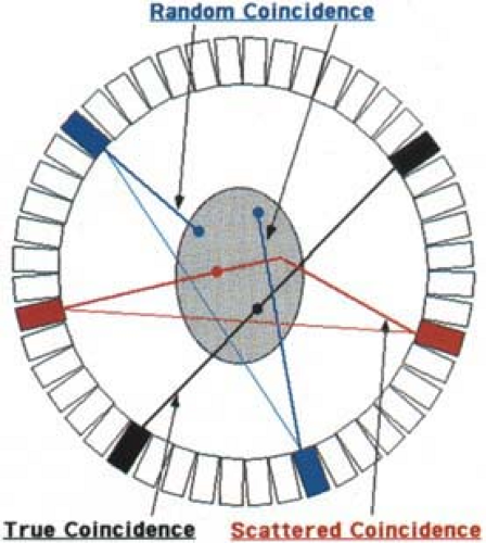 Figure 5.5. Random and scattered coincidences. One would like each detected coincidence event to correctly identify a line of response passing through the point of positron decay. For this to occur both 511 keV photons need to be detected and neither photon can be scattered in tissue. The black dot, detectors, and connecting line of response depict such a “true” coincidence event. If only one photon is detected from each of two positron decays and these are detected with the coincidence resolving time, a “random” or accidental coincidence is said to have occurred. This is depicted by the two blue dots and detectors. The two thicker blue lines indicate the path of the two detected photons, while the thinner blue line corresponds to the line of response that is recorded for this “random” coincidence event. Note that this line does not pass through either of the two points and therefore causes misplacement of the coincidence event and hence error in the reconstructed image. If both photons from a single decay are detected but one (or both) photons are scattered in the body prior to detection, the coincidence event also is misplaced as shown by the red dot, detectors, and lines. The two thicker red lines indicate the actual paths taken by the two photons, while the thinner red line indicates the line of response that is recorded for this “scattered” coincidence event. Again, the line does not pass through the point of decay and causes error in the reconstructed image. |
The second method involves setting up two distinct coincidence windows. The first window is the standard coincidence window of width τ. As before, both true and random coincidences are recorded in this window, which for this approach is called the prompt coincidence window. A second coincidence circuit is set up, but with one of the two inputs being delayed by a time considerably greater than the resolving time, τ. Rather than searching for two events that occur within a single 10-nanosecond window (as is done in the prompt circuit), this circuit, in effect, searches for events that occur in two separate 10-nanosecond windows offset by, for example, 100 nanoseconds. This offset window produces what are called delayed coincidence events. The probability that a true coincidence occurs in the delayed window is zero, while the probability that a random coincidence occurs is the same as in the prompt window. Thus, the prompt window records true plus random coincidences, while the delayed window records only randoms. Subtracting delayed from prompt coincidences yields an estimate of true coincidences. The advantage of this approach is that it can be implemented online and requires no postacquisition processing. During data acquisition, a memory location exists for each detector pair whose projection ray subtends the FOV. For every prompt coincidence event detected, the memory location representing the appropriate projection ray is incremented by 1. For each delayed event detected, the memory location is decremented by 1. This commonly used decrementing procedure ruins the Poisson statistical model that is the theoretical basis for Equation 5.13 and the MLEM (and OSEM) iterative reconstruction algorithms. Alternative reconstruction methods have been proposed for PET measurements that are precorrected for random coincidences (54,55).
Scattered Coincidence Events
At 511 keV energies, two types of photon interactions occur: Compton scattering and photoelectric absorption. As discussed in Chapter 3, scintillation detectors are designed to maximize the number of photoelectric interactions, while minimizing the probability of Compton scattering. This is accomplished by a material with a high effective atomic number and high density. However, due to the lower effective atomic number in the body, most interactions in human tissue occur via Compton scattering, as depicted in Fig. 5.5. As was the case for random coincidence events, detection of events where one or both of the photons have undergone at least one Compton scatter causes the location of the annihilation to be misplaced. Inclusion of scattered events causes a relatively uniform background, decreasing image contrast and reducing SNR. Naturally we would like to record only unscattered photon events, but is not possible to identify with complete certainty whether a particular event is scattered. Scintillation detectors with higher light output do, however, have better energy resolution and thus are better able to distinguish unscattered from scattered events.
Accurate correction for Compton scattered photons is extremely complex with hundreds of papers having been written on quantifying its effects as well as developing and testing methods for correction. For 2D acquisition, scatter was only moderately important with 15% to 20% of the detected events being scattered. Image quality was not affected greatly, hence scatter correction was often ignored without major impact. With 3D scanning, 35% to 50% of the detected events may be scattered, and correction has become much more critical. Current scatter corrections fall into three basic groups: (a) those using multiple energy windows; (b) those based on direct calculation from analytic formulas for Compton scatter or on Monte Carlo calculations; and (c) methods involving a variety of techniques such as convolution, deconvolution, or the fitting of analytic functions to areas of the image void of radioactivity (thus representing only scattered events).
Although each of these three general techniques has its own advantages and limitations, details of such methods are beyond the scope of this chapter. The reader is referred to Bailey et al. (56) for a more thorough discussion of scattered events and correction methods to account their occurrence. This chapter describes briefly only the direct calculation approach. It is assumed that the true radioactivity distribution can be reconstructed accurately when the measured PET data, emission and transmission, contain only unscattered events. The measured PET data, however, include both true and scattered events. The correction is performed iteratively. The original measured data are reconstructed as an initial estimate of the true radioactivity distribution. From these images and the analytic formulas for Compton scatter, the scatter component to the raw projection data is estimated. This scatter component is subtracted from the measured PET data as the next approximation to
the scatter-free projection data. This new projection set is reconstructed as the next approximation to the true radioactivity distribution. These steps are repeated until the images reconstructed from the current estimate of the scatter-free projection data yield predicted scatter that when added to the scatter-free data equal the measured projection data. In practice, successive approximations to the scatter-free distribution can be made during the normal iterations of the OSEM reconstruction algorithm.
the scatter-free projection data. This new projection set is reconstructed as the next approximation to the true radioactivity distribution. These steps are repeated until the images reconstructed from the current estimate of the scatter-free projection data yield predicted scatter that when added to the scatter-free data equal the measured projection data. In practice, successive approximations to the scatter-free distribution can be made during the normal iterations of the OSEM reconstruction algorithm.
Attenuation
A final but extremely important correction to the projection data is that which accounts for the effects of photon attenuation in the body. For a true coincidence event to be detected, both photons must exit the body. This is less likely for annihilations located deep within the body than for ones occurring near the body’s surface. One convenient aspect of PET imaging is that the attenuation correction factor for any given projection ray is the same for a positron annihilation occurring anywhere along the ray. The net attenuation is simply the product of the probabilities that each photon escapes without interacting:
where μ is the linear attenuation coefficient for 511 keV photons in tissue, and x1,2 are the distances the two photons must travel through tissue. Since the sum x1 + x2 always equals the total path length, l, through the body, the attenuation correction factor is given by e+μl. Independence of the position of the annihilation along the ray is true even if the attenuation coefficient varies across the path due to multiple tissue types (lung, soft tissue, and bone).
Again, there are two general approaches used to account for photon attenuation. First is a calculated or analytic method, where the path length for each projection ray is estimated in some fashion and the value for μ is assumed. The attenuation correction factor, as indicated above, is simply e+μl. The two main limitations of this approach are: (a) it is not always easy to determine the path length of all projection rays, and (b) variations in μ are not easily accounted for. A major advantage is there is no statistical noise associated with the correction. This approach has been used for brain imaging where the shape of the head can be approximated by an ellipse and the attenuation is uniform except for a thin rim of skull.
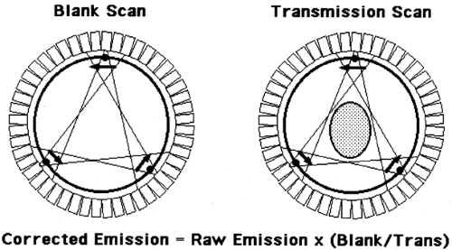 Figure 5.6. Schematic for measured attenuation correction. As described in the text, measured attenuation is performed by acquiring two scans: a “blank” scan and a “transmission” scan. Both scans are performed using radioactive sources that are rotated around the gantry in front of the detectors. The blank scan measures the coincidence rate from the sources when nothing is in the field of view. The transmission scan measures the coincidence rate when the object being imaged is in the field of view. The ratio between these two measures is used, ray by ray, to correct the emission projection data. |
A second method is to measure the attenuation factors directly. This approach typically uses external rod sources that are rotated around the FOV, until recently being replaced by CT scanning approaches (see Chapter 2). Most sources contain the positron-emitter 68Ge, which has a 0.75-year half-life. Two scans are acquired as shown in Fig. 5.6, a blank scan, which is acquired with nothing in the FOV (similar in nature to the normalization scan described above), and a transmission scan, where the subject is in the FOV in the identical position as the emission scan. After appropriate corrections, the ratio of the measured projection data from the blank scan divided by the transmission scan yields a correction factor for the emission data. If a particular projection ray has 400 counts in the blank scan, but only 50 counts in the transmission scan, the correction factor for the emission data will be 8.
Although measured attenuation avoids the problems associated with the analytic approach, several other potential problems arise. Statistical uncertainty in the blank and particularly the transmission scan propagates into the reconstructed emission images. This problem is particularly bad in the abdomen (especially with large abdomens) where attenuation is high and thus detected transmission events low. Subject motion between the times of the transmission and emission scans can cause significant errors in the correction factors for particular projection rays, resulting in severe artifacts when motion is substantial. Such artifacts are considerably worse for filtered back-projection than for iterative approaches. Transmission scans also take considerable time. If a subject can reasonably be expected to remain still for 1 to 2 hours, we would want to spend the entire time acquiring emission data. For body scans, however, nearly as much time is required for transmission as emission imaging. Furthermore, for clinical FDG scans that have a 50-minute or longer tracer-uptake period, it becomes problematic to perform all transmission scanning prior to injection of the radiotracer. This is due to both subject motion and study duration issues. If transmission scans are performed postinjection, then the contribution of the FDG events to transmission data must be taken into account.
Over the past decade much work has been done to improve attenuation correction. The two most significant advances are described here. The first was to provide the capability of performing postinjection transmission scans. Prior to this advance, a typical clinical protocol might include 30 minutes of transmission scanning, injection of [18F]-FDG, and then a 50-minute uptake period
followed by 30 to 60 minutes or more of emission imaging. Thus, a subject would have to lie still for more than 2 hours. This is both difficult on the patient and it occupies the scanner for long periods of time even when no data are being acquired. Furthermore, registration between transmission and emission scans may be jeopardized by the length of time between the acquisitions. Through the use of rotating rod sources instead of a continuous ring of radioactivity, postinjection transmission scanning is possible. For discrete rod sources, only a small fraction of the projection rays contain valid transmission coincidences at any given time. Only rays that pass through one of the rod sources can have coincidences that originate from within the rod. All other events come from FDG decay. Thus, the majority of emission coincidences that occur at any given time are rejected based on the known positions of the rods.
followed by 30 to 60 minutes or more of emission imaging. Thus, a subject would have to lie still for more than 2 hours. This is both difficult on the patient and it occupies the scanner for long periods of time even when no data are being acquired. Furthermore, registration between transmission and emission scans may be jeopardized by the length of time between the acquisitions. Through the use of rotating rod sources instead of a continuous ring of radioactivity, postinjection transmission scanning is possible. For discrete rod sources, only a small fraction of the projection rays contain valid transmission coincidences at any given time. Only rays that pass through one of the rod sources can have coincidences that originate from within the rod. All other events come from FDG decay. Thus, the majority of emission coincidences that occur at any given time are rejected based on the known positions of the rods.
The second major advance was the development of a combination calculated/measured attenuation correction that makes use of the advantages of each approach. A transmission scan is acquired, but rather than performing the correction based on the ray-by-ray difference between blank and transmission data, this scan is reconstructed into a map of attenuation coefficients. Although individual rays are noisy, the reconstructed transmission image allows segmentation into different tissue types. Each pixel of the image is assigned an attenuation coefficient based on the segmentation. The segmented images, in practice, are smoothed and then used to calculate attenuation factors for the emission data. This process greatly reduces noise propagation from the transmission measurements into the reconstructed emission images. Fig. 5.7 shows a 2D whole-body transaxial slice reconstructed with measured attenuation (left) and with segmented attenuation correction (right). Clearly demonstrated is the noise propagation from the transmission data into the emission image when attenuation correction is performed without segmentation. In addition, reconstructions were performed with both FBP (top) and with an iterative OSEM algorithm (bottom). The better noise properties of iterative reconstruction are demonstrated clearly. In particular, notice the reduction in streak artifacts with OSEM that plague back- projection techniques. Keeping in mind that both images are derived from the identical projection data, the improvement from the upper left image to the lower right image (which has both segmented attenuation correction and iterative reconstruction) truly is impressive. A variety of additional issues arise when determining attenuation corrections for 3D PET. A major difficulty is that the radioactivity level of the rod sources required for adequate statistics in 2D studies causes excessive dead time and random coincidence
rates in 3D studies. Currently, transmission scans are performed in 2D mode, reconstructed, and then forward projected into the full set of 3D projection rays. Considerable work by Erdogan and Fessler et al. (57,58) has been performed to maximize the quality of the reconstructed transmission data.
rates in 3D studies. Currently, transmission scans are performed in 2D mode, reconstructed, and then forward projected into the full set of 3D projection rays. Considerable work by Erdogan and Fessler et al. (57,58) has been performed to maximize the quality of the reconstructed transmission data.
Related posts:
Stay updated, free articles. Join our Telegram channel

Full access? Get Clinical Tree


