Deformable Image Registration

Fig. 1

Typical components of registration algorithms

The choice of the transformation model is usually dictated by the application at hand and is related to the nature of the deformation to be recovered. High-dimensional nonlinear models are necessary to cope with highly variable soft tissue, while low degrees of freedom models can represent the mapping between

rigid bone structures. It is important to note that increasing the degrees of freedom of the model, and thus enriching its descriptive power, often comes at the cost of increased computational burden.

Several transformation models have been introduced in medical imaging for non-rigid alignment. These models can be coarsely classified into two categories (see Fig. 1 [30, 75]): i) models derived from physical models, and ii) models derived from the interpolation theory or geometric models. Among the most prominent choices of the first class, one may cite elastic [19, 20], fluid [14, 18] or diffusion models [22, 80, 85]. Whereas, the second class comprises radial basis functions [10, 67], free-form deformations [68, 69], locally affine [55] and poly-affine models [2], or models parametrized by Fourier [1, 4] or Wavelet basis functions [87].

The similarity criterion quantifies the degree of alignment between the images. Registration methods can be classified into three categories (see Fig. 1) depending on the type of information that is utilized by the similarity criterion: i) geometric registration (a.k.a.landmark/feature-based registration); ii) iconic registration (a.k.a.voxel-wise registration); and iii) hybrid registration.

Geometric registration aims to align meaningful anatomical locations or salient landmarks, which are either automatically extracted from the images [51] or provided by an expert. Geometric information is typically represented as point-sets and registration is tackled by first estimating the point correspondences [43, 82] and then employing an interpolation strategy (e.g. thin-plate splines [10]) to determine a dense deformation field that will align the images. Alternatively, geometric methods may infer directly the transformation that aligns the images without explicitly estimating point correspondences. This is possible by representing geometric information either as probability distributions [23, 83] or through the use of signed distance transformations [32]. Last, there exist methods that opt to simultaneously solve for both the correspondences and the transformation [15].

Iconic methods employ a similarity criterion that takes into account the intensity information of all image elements. The difficulty of choosing an appropriate similarity criterion varies greatly depending on the problem. In the mono-modal case, where both images are acquired using the same device and one can assume that the intensity profiles for the two images differ only by Gaussian noise, the use of sum of squared differences can be sufficient. Nonetheless, in the multi-modal case, where images from different modalities are involved, the criterion should be able to account for the different principles behind the acquisition protocols and capture the relation between the distinct intensity profiles. Towards this end, criteria based on statistics and information theory have been proposed. Examples include correlation ratio [65], mutual-information [52, 86] and Kullback-Leibler divergence [16]. Last, attribute-based methods that construct rich descriptions by summarizing intensity information over local regions have been proposed for both mono-modal and multi-modal registration [48, 62, 74].

Hybrid methods opt to exploit both iconic and geometric information in an effort to leverage their complementary nature towards more robust and accurate registration. Depending on how one combines the two types of information, three subclasses can be distinguished. In the first case, geometric information is used to initialize the alignment, while intensity-based volumetric registration refines the results [35, 64]. In the second case, geometric information can be used to provide additional constraints that are taken into account during iconic registration [27, 29]. In the third case, iconic and geometric information are integrated in a single objective function that allows for the simultaneous solution of both problems [11, 25, 76].

Once the transformation model and a suitable similarity criterion have been defined, an optimization method is used in order to infer the optimal set of parameters by maximizing the alignment of the two images. Solving for the optimal parameters is particularly challenging in the case of image registration. The reason behind this lies in the fact that image registration is, in general, an ill-posed problem and the associated objective functions are typically non-linear and non-convex. The optimization methods that are typically used in image registration fall under the umbrella of either continuous or discrete methods.

Typically, continuous optimization methods are constrained to problems where the variables take real values and the objective function is differentiable. This type of problems are common in image registration. As a consequence, these methods (typically gradient descent approaches) have been widely used in image registration [8, 69] because of the fact that they are rather intuitive and easy to implement. Moreover, they can handle a wide class of objective functions allowing for complex modeling assumptions regarding the transformation model. Nonetheless, they are often sensitive to the initial conditions, while being non-modular with respect to the similarity criterion and the transformation model. What is more, they are often computationally inefficient [24].

On the other hand, discrete optimization methods tackle problems where the variables take discrete values. Discrete optimization methods based on the Markov Random Field theory have been recently investigated in the context of image registration [24, 25]. Discrete optimization methods are constrained by limited precision due to the necessary quantization of the solution space. Moreover, they can not efficiently model complex variable interactions due to increased difficulty in inference. However, recent advances in higher-order inference methods have allowed the modeling of more sophisticated regularization priors [42]. More importantly, discrete optimization methods are versatile and can handle a wide range of similarity metrics (including non-differentiable ones). What is more, they are more robust to the initial conditions due to the global search they perform, while often converging faster than continuous methods.

In this chapter, we review the application of Markov Random Fields (MRFs) in deformable image registration. We explain in detail how one can map image registration from the continuous domain to discrete graph structures. We first present graph-based deformable registration in the case of iconic registration and show how one can encode intensity-based and statistical approaches. We then present discrete attribute-based registration methods and complete the presentation by describing MRF models for geometric and hybrid registration. Throughout this chapter, we discuss the underlying assumptions as well as implementation details. Experimental results that demonstrate the value of graph-based registration are given at the end of every section.

2 Graph-based Iconic Deformable Registration

In this chapter, we focus on pairwise deformable registration. The two images are usually termed as source (or moving) and target (or fixed) images, respectively. The source image is denoted by $S:\varOmega _{S} \subset \mathbb{R}^{d}\mapsto \mathbb{R}$ , while the target image by $T:\varOmega _{T} \subset \mathbb{R}^{d}\mapsto \mathbb{R}$ , d = { 2, 3}. Ω _Sand Ω _Tdenote the image domain for the source and target images, respectively. The source image undergoes a transformation $\mathcal{T}:\varOmega _{S}\mapsto \varOmega _{T}$ .

Image registration aims to estimate the transformation $\mathcal{T}$ such that the two images get aligned. This is typically achieved by means of an energy minimization problem:

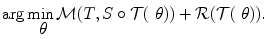
$\displaystyle{ \arg \min _{\mbox{ $\theta $}}\mathcal{M}(T,S \circ \mathcal{T} (\mbox{ $\theta $})) + \mathcal{R}(\mathcal{T} (\mbox{ $\theta $})). }$

(1)

Thus, the objective function comprises two terms. The first term, $\mathcal{M}$ , quantifies the level of alignment between a target image T and a source image S under the influence of the transformation $\mathcal{T}$ parametrized by $\mbox{ $\theta $}$ . The second term, $\mathcal{R}$ , regularizes the transformation and accounts for the ill-posedness of the problem. In general, the transformation at every position $\mathbf{x} \in \varOmega$ (Ω depicting the image domain) is given as $\mathcal{T} (\mathbf{x}) = \mathbf{x} + \mathbf{u}(\mathbf{x})$ where $\mathbf{u}$ is the deformation field.

The previous minimization problem can be solved by adopting either continuous or discrete optimization methods. In this chapter, we focus on the application of discrete methods that exploit Markov Random Field theory.

2.1 Markov Random Fields

In discrete optimization settings, the variables take discrete values and the optimization is formulated as a discrete labeling problem where one searches to assign a label to each variable such that the objective function is minimized. Such problems can be elegantly expressed in the language of discrete Markov Random Field theory.

An MRF is a probabilistic model that can be represented by an undirected graph $\mathcal{G} = \left (\mathcal{V},\mathcal{E}\right )$ . The set of vertices $\mathcal{V}$ encodes the random variables, which take values from a discrete set $\mathcal{L}$ . The interactions between the variables are encoded by the set of edges $\mathcal{E}$ . The goal is to estimate the optimal label assignment by minimizing an energy of the form:

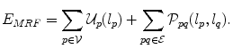
$\displaystyle{ E_{MRF} =\sum _{p\in \mathcal{V}}\mathcal{U}_{p}(l_{p}) +\sum _{pq\in \mathcal{E}}\mathcal{P}_{pq}(l_{p},l_{q}). }$

(2)

The MRF energy also comprises two terms. The first term is the sum of all unary potentials $\mathcal{U}_{p}$ of the nodes $p \in \mathcal{V}$ . This term typically corresponds to the data term since the unary terms are usually used to encode data likelihoods. The second term comprises the pairwise potentials $\mathcal{P}_{pq}$ modeled by the edges connecting nodes p and q. The pairwise potentials usually act as regularizers penalizing disagreements in the label assignment of tightly related variables.

Many algorithms have been proposed in order to perform inference in the case of discrete MRFs. In the works that are presented in this chapter, the fast-PD¹ algorithm [39, 40] has been used to estimate the optimal labeling. The main motivation behind this choice is its great computational efficiency. Moreover, the fast-PD algorithm is appropriate since it can handle a wide-class of MRF models allowing us to use different smoothness penalty functions and has good optimality guarantees.

In the continuation of this section, we detail how deformable registration is formulated in terms of Markov Random Fields. First, however, the discrete formulation requires a decomposition of the continuous problem into discrete entities. This is described below.

2.2 Decomposition into Discrete Deformation Elements

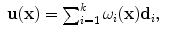
Without loss of generality, let us consider a grid-based deformation model that combines low degrees of freedom with smooth local deformations. Let us consider a set of k control points distributed along the image domain using a uniform grid pattern. Furthermore, let k be much smaller than the number of image points. One can then deform the embedded image by manipulating the grid of control points. The dense displacement field is defined as a linear combination of the control point displacements $\mathbf{D} =\{ \mathbf{d}_{1},...,\mathbf{d}_{k}\}$ , with $\mathbf{d}_{i} \in \mathbb{R}^{d}$ , as:

$\displaystyle\begin{array}{rcl} \mathbf{u}(\mathbf{x}) =\sum _{ i=1}^{k}\omega _{ i}(\mathbf{x})\mathbf{d}_{i},& &{}\end{array}$

(3)

and the transformation $\mathcal{T}$ becomes:

$\displaystyle\begin{array}{rcl} \mathcal{T} (\mathbf{x}) = \mathbf{x} +\sum _{ i=1}^{k}\omega _{ i}(\mathbf{x})\mathbf{d}_{i}.& &{}\end{array}$

(4)

ω _icorresponds to an interpolation or weighting function which determines the influence of a control point i to the image point x – the closer the image point the higher the influence of the control point. The actual displacement of an image point is then computed via a weighted sum of control point displacements. A dense deformation of the image can thus be achieved by manipulating these few control points.

The free-form deformation is a typical choice for such a representation [71]. This model employs a weighting scheme that is based on cubic B-splines and has found many applications in medical image registration [69] due to its efficiency and the local support of the control points. We also employ this model. Nonetheless, let us note that the discrete deformable registration framework is modular with respect to the interpolation scheme and one may use this preferred strategy.

The parametrization of the deformation field leads naturally to the definition of a set of discrete deformation elements. Instead of seeking a displacement vector for every single image point, now, only the displacement vectors for the control points need to be sought. If we take them into consideration, the matching term (see Eq. (1)) can be rewritten as:

$\displaystyle{ \mathcal{M}(S \circ \mathcal{T},T) = \frac{1} {k}\sum _{i=1}^{k}\int _{ \varOmega _{S}}\hat{\omega }_{i}(\mathbf{x})\,\rho (S \circ \mathcal{T} (\mathbf{x}),T(\mathbf{x}))d\mathbf{x}, }$

(5)

where $\hat{\omega }_{i}$ are weighting functions similar to the ones in Eq. (4) and ρ denotes a similarity criterion.

Here, the weightings determine the influence or contribution of an image point x onto the (local) matching term of individual control points. Only image points in the vicinity of a control point are considered for the evaluation of the intensity-based similarity measure with respect to the displacement of this particular control point. This is in line with the local support that a control point has on the deformation. The previous is valid when point-wise similarity criteria are considered. When a criterion based on statistics or information theory is used, a different definition of $\hat{\omega }_{i}$ is adopted,

$\displaystyle{ \hat{\omega }_{i}(\mathbf{x}) = \left \{\begin{array}{@{}l@{\quad }l@{}} 1,\quad &\mathrm{if}\ \omega _{i}(\mathbf{x}) \geq 0,\\ 0 \quad &\mathrm{otherwise. } \end{array} \right. }$

(6)

Thus, in both cases the criterion is evaluated on a patch. The only difference is that the patch is weighted in the first case. These local evaluations enhance the robustness of the algorithm to local intensity changes. Moreover, they allow for computationally efficient schemes.

The regularization term of the deformable registration energy (Eq. (1)) can also be expressed on the basis of the set of control points as:

$\displaystyle{ \mathcal{R} = \frac{1} {k}\sum _{i=1}^{k}\int _{ \varOmega _{S}}\hat{\omega }_{i}(\mathbf{x})\,\psi (\mathcal{T} (\mathbf{x}))d\mathbf{x}, }$

(7)

where ψ is a function that promotes desirable properties of the dense deformation field such as the smoothness and topology preservation.

2.3 Markov Random Field Registration Energy

Having identified the discrete deformation elements of our problem, we need to map them to MRF entities, i.e., the graph vertices, the edges, the set of labels, and the potential functions.

Let $\mathcal{G}_{\text{ico}}$ denote the graph that represents our problem. In this case, the random variables of interest are the control point displacement updates. Thus, the set of vertices $\mathcal{V}_{\text{ico}}$ is used to encode them, i.e., $\vert \mathcal{V}_{\text{ico}}\vert = \vert \varDelta \mathbf{D}\vert = k$ . Moreover, assigning a label $l_{p} \in \mathcal{L}_{\text{ico}}$ to a node $p \in \mathcal{V}_{\text{ico}}$ is equivalent to displacing the corresponding control point p by an update Δ d _p, or $l_{p} \equiv \varDelta \mathbf{d}_{p}$ . In other words, the label set for this set of variable is a quantized version of the displacement space ( $L_{\text{ico}} \subset \mathbb{R}^{d}$ ). The edge system $\mathcal{E}_{\text{ico}}$ is constructed by following either a 6-connected neighborhood system in the 3D case, or a 4-connected system in the 2D case. The edge system follows the grid structure of the transformation model.

According to Eq. (5) we define the unary potentials as:

$\displaystyle\begin{array}{rcl} \mathcal{U}_{\text{ico},p}(l_{p}) =\int _{\varOmega _{S}}\hat{\omega }_{p}(\mathbf{x})\,\rho (S \circ \mathcal{T}_{\text{ico},l_{ p}}(\mathbf{x}),T(\mathbf{x}))\,d\mathbf{x},& &{}\end{array}$

(8)

where $\mathcal{T}_{\text{ico},l_{ p}}$ denotes the transformation where a control point p has been updated by l _p. Region-based and statistical measures are again encoded in a similar way based on a local evaluation of the similarity measure.

Conditional independence is assumed between the random variables. As a consequence, the unary potential that constitutes the matching term can only be an approximation to the real matching energy. That is because the image deformation, and thus the local similarity measure, depends on more than one control point since their influence areas do overlap. Still, the above approximation yields very accurate registration as deomonstrated by the experimental validation results that are reported in latter sections (Sect. 2.4, Sect. 3.3 and Sect. 4.3). Furthermore, it allows an extremely efficient approximation scheme which can be easily adapted for parallel architectures yielding extremely fast cost evaluations.

Actually, the previous approximation results in a weighted block matching strategy encoded on the unary potentials. The smoothness of the transformation derives from the explicit regularization constraints encoded by the pairwise potentials and the implicit smoothness stemming from the interpolation strategy.

The evaluation of the unary potentials for a label $l \in \mathcal{L}_{\text{ico}}$ corresponding to an update Δ d can be efficiently performed as follows. First, a global translation according to the update Δ d is applied to the whole image, and then the unary potentials for this label and for all control points are calculated simultaneously. This results in an one pass through the image to calculate the cost and distribute the local energies to the control points. The constrained transformation in the unary potentials is then simply defined as $\mathcal{T}_{\text{ico},l_{ p}}(\mathbf{x}) = \mathcal{T}_{\text{ico}}(\mathbf{x}) + l_{p}$ , where $\mathcal{T}_{\text{ico}}(\mathbf{x})$ is the current or initial estimate of the transformation.

The regularization term defined in Eq. (7) could be defined as well in the above manner. However, this is not very efficient since the penalties need to be computed on the dense field for every variable and every label. If we consider an elastic-like regularization, we can employ a very efficient discrete approximation of this term based on pairwise potentials as:

$\displaystyle\begin{array}{rcl} \mathcal{P}_{\text{ico,elastic},pq}(l_{p},l_{q}) = \frac{\|(\mathbf{d}_{p} +\varDelta \mathbf{d}_{p}) - (\mathbf{d}_{q} +\varDelta \mathbf{d}_{q})\|} {\|\mathbf{p} -\mathbf{q}\|}.& &{}\end{array}$

(9)

The pairwise potentials penalize deviations of displacements of neighboring control points $(p,q) \in \mathcal{E}_{\text{ico}}$ which is an approximation to penalizing the first derivatives of the transformation. Recall that $l_{p} \equiv \varDelta \mathbf{d}_{p}$ . Note, we can also remove the current displacements d _pand d _qfrom the above definition yielding a term that only penalizes the updates on the deformation. This would change the behavior of the energy from an elastic-like to a fluid-like regularization.

Let us detail how the label set $\mathcal{L}_{ico}$ is constructed since that entails an important accuracy-efficiency trade-off. The smaller the set of labels, the more efficient is the inference. However, few labels result in a decrease of the accuracy of the registration. This is due to the fact that the registration accuracy is bounded by the range of deformations covered in the set of labels. As a consequence, it is reasonable to assume that the registration result is sub-optimal. In order to strike a satisfactory balance between accuracy and efficiency, we opt for an iterative labeling strategy combined with a search space refinement one. At each iteration, the optimal labeling is computed yielding an update on the transformation, i.e. $l_{p} \equiv \varDelta \mathbf{d}_{p}$ . This update is applied to the current estimate, and the subsequent iteration continues the registration based on the updated transformation and a refined label set. Thus, the error induced by the approximation stays small and incorrect matches can be corrected in the next iteration. Furthermore, the overall domain of possible deformations is rather bounded by the number of iterations and not by the set of finite labels.

The iterative labeling allows us to keep the label set quite small. The refinement strategy on the search space is rather intuitive. In the beginning we aim to recover large deformations and as we iterate, finer deformations will be added refining the solution. In each iteration, a sparse sampling with a fixed number of samples s is employed. The total number of labels in each iteration is then $\vert \mathcal{L}_{\text{ico}}\vert \! =\! g \cdot s + 1$ including the zero-displacement and g is the number of sampling directions. We uniformly sample displacements along certain directions up to a maximum displacement magnitude d _max. Initially, the maximum displacement corresponds to our estimation of the larger deformation to be recovered. In the subsequent iterations, it is decreased by a user-specified factor 0 < f < 1 limiting and refining the search space.

The number and orientation of the sampling directions g depend on the dimensionality of the registration. One possibility is to sample just along the main coordinate axes, i.e. in positive and negative direction of the x-, y-, and z-axis (in case of 3D). Additionally, we can add samples for instance along diagonal axes. In 2D we commonly prefer a star-shape sampling, which turns out to be a good compromise between the number of samples and the sampling density. In our experiments we found that also very sparse samplings (e.g., just along the main axes) gives very accurate registration results but might increase the total number of iterations that are needed until convergence. However, a single iteration is much faster to compute when the label set is small. In all our experiments we find that small label sets provide an excellent performance in terms of computational speed and registration accuracy.

The explicit control that one has over the creation of the label set $\mathcal{L}$ enables us to impose desirable properties on the obtained solution without further modifying the discrete registration model. Two interesting properties that can be easily enforced by adapting appropriately the discrete solution space are diffeomorphisms and symmetry. Both properties are of particular interest in medical imaging and have been the focus of the work of many researchers.

Diffeomorphic transformations preserve topology and both they and their inverse are differentiable. These transformations are of interest in the field of computational neuroanatomy. Moreover, the resulting deformation fields are, in general, more physically plausible since foldings, which would disrupt topology, are avoided. As a consequence, many diffeomorphic registration algorithms have been proposed [3, 5, 8, 68, 85].

In this discrete setting, it is straightforward to guarantee a diffeomorphic result through the creation of the label set. By bounding the maximum sampled displacement by 0. 4 times the deformation grid spacing, the resulting deformation is guaranteed to be diffeomorphic [68].

The majority of image registration algorithms are asymmetric. As a consequence, when interchanging the order of input images, the registration algorithm does not estimate the inverse transformation. This asymmetry introduces undesirable bias upon any statistical analysis that follows registration because the registration result depends on the choice of the target domain. Symmetric algorithms have been proposed in order to tackle this shortcoming [5, 13, 56, 79, 84].

Symmetry can also be introduced in graph-based deformable registration in a straightforward manner [77]. This is achieved by estimating two transformations, $\mathcal{T}^{f}$ and $\mathcal{T}^{b}$ , that deform both the source and the target images towards a common domain that is constrained to be equidistant from the two image domains. In order for this to be true, the transformations, or equivalently the two update deformation fields, should sum up to zero. If one assumes a transformation model that consists of two isomoprhic deformation grids, this constraint translates to ensuring that the displacement updates of corresponding control points in the two grips sum to zero and can be simply mapped to discrete elements.

The satisfaction of the previous constraint can be easily guaranteed in a discrete setting by appropriately constructing the label set. More specifically, by letting the labels index pairs of displacement updates (one for each deformation field) that sum to zero, i.e. $l_{p} \equiv \{\varDelta \mathbf{d}_{p}^{f},-\varDelta \mathbf{d}_{p}^{b}\}$ . The extension of the unary terms is also straightforward, while the pairwise potentials and the graph construction are the same.

2.4 Experimental Validation

In this section, we present experimental results for the graph-based symmetric registration in 3D brain registration. The data set consists of 18 T1-weighted brain volumes that have been positionally normalized into the Talairach orientation (rotation only). The MR brain data set along with manual segmentations was provided by the Center for Morphometric Analysis at Massachusetts General Hospital and are available online². The data set was rescaled and resampled so that all images have a size equal to 256 × 256 × 128 and a physical resolution of approximately 0. 9375 × 0. 9375 × 1. 5000 mm.

This set of experiments is based on intensity-based similarity metrics (for results using attribute-based similarity metrics, we refer the reader to the next section of this chapter). The results are compared with a symmetric registration method based on continuous optimization [5] that is considered to be the state of the art in continuous deformable registration [38]. Both methods use Normalized Cross Correlation as the similarity criterion.

A multiresolution scheme was used in order to harness the computational burden. A three-level image pyramid was considered while a deformation grid of four different resolutions was employed. The two finest grid resolutions operated on the finest image resolution. The two coarsest operated on the respective coarse image representations. The initial grid spacing was set to 40 mm resulting in a deformation grid of size 7 × 7 × 6. The size of the gird was doubled at each finer resolution. A number of 90 labels, 30 along each principal axis, were used. The maximum displacement indexed by a label was bounded to 0.4 times the grid spacing. The pairwise potentials were weighted by a factor of 0.1.

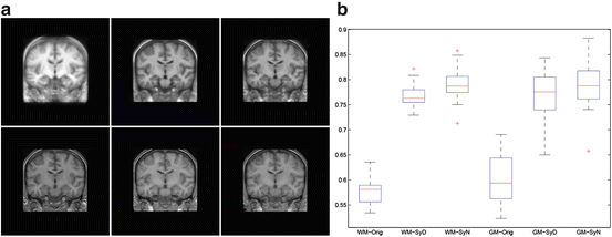
Fig. 2

a) In the first row, from left to right, the mean intensity image is depicted for the data set, after the graph-based symmetric registration method and after [5]. In the second row, from left to right, the target image is shown as well as a typical deformed image for the graph-based symmetric registration method and [5]. For all cases, the central slice is depicted. b) Boxplots for the DICE criterion initially, with the graph-based symmetric registration method and with [5]. On the left, the results for the WM. On the right, the results for the GM. The figure is reprinted from [77]

The qualitative results (sharp mean and deformed image) suggest that both methods successfully registered the images to the template domain. The results of [5] seem to have produced more aggressive deformation fields that have resulted to some unrealistic deformations in the top of the brain and can also be observed in the borders between white matter (WM) and gray matter (GM). This aggressive registration has also resulted in slightly more increased DICE coefficients for WM and GM. However, the results reported for the graph-based registration method were obtained in 10 min. On the contrary, 1 hour was necessary to register the images with [7] approximately. This important difference in the computational efficiency between the two methods can outweigh the slight difference in the quality of the solution in practice.

3 Graph-based Attribute-Based Deformable Registration

In the previous section, we studied the application of intensity-based deformable registration methods that involve voxel-wise and statistical similarity criteria. While these criteria are easy to compute and widely used, they suffer from certain shortcomings. First, they often have difficulties to reflect the underlying anatomy because pixels belonging to the same anatomical structure are often assigned different intensity values due to variabilities arising from scanners, imaging protocols, noise, partial volume effects, contrast differences, and image inhomogeneities. Moreover, single intensities are not informative enough to uniquely characterize image elements, and thus reliably guide image registration. For instance, hundreds of thousands of gray matter voxels in a brain image share similar intensities; but they belong to different anatomical structures. As a consequence, matching ambiguities arise in the matching between two images.

Only gold members can continue reading. Log In or Register to continue