is often chosen to be a signed distance function of the embedded contour(s). Such a signed distance function can be computed very efficiently using the fast marching method [94, 109] or the fast sweeping method [130].
For image segmentation problems, a GDM is either formulated as an energy minimization problem where the solution is sought through gradient descent optimization, or by directly designing the various forces that drive the model contour(s) towards desired object boundaries. In either case, the final evolution equation regarding the level set function Φ(x, t) can be summarized in the following general form:
![$$\displaystyle{\frac{\partial \varPhi (\mathbf{x},t)} {\partial t} = [F_{\mathrm{prop}}(\mathbf{x},t) + F_{\mathrm{curv}}(\mathbf{x},t)]\vert \nabla \varPhi (\mathbf{x},t)\vert +\boldsymbol{ F}_{\mathrm{adv}}(\mathbf{x},t) \cdot \nabla \varPhi (\mathbf{x},t),}$$](/wp-content/uploads/2016/09/A151032_1_En_5_Chapter_Equa.gif) where F prop, F curv, and F adv are spatially-varying force terms that drive the front evolution. In particular, F prop is an expansion or contraction force, F curv is the part of the force that depends on the intrinsic geometry, especially the curvature of the implicit contour and/or its derivatives, and F adv is an advection force that passively transports the contour.
where F prop, F curv, and F adv are spatially-varying force terms that drive the front evolution. In particular, F prop is an expansion or contraction force, F curv is the part of the force that depends on the intrinsic geometry, especially the curvature of the implicit contour and/or its derivatives, and F adv is an advection force that passively transports the contour.
![$$\displaystyle{\frac{\partial \varPhi (\mathbf{x},t)} {\partial t} = [F_{\mathrm{prop}}(\mathbf{x},t) + F_{\mathrm{curv}}(\mathbf{x},t)]\vert \nabla \varPhi (\mathbf{x},t)\vert +\boldsymbol{ F}_{\mathrm{adv}}(\mathbf{x},t) \cdot \nabla \varPhi (\mathbf{x},t),}$$](/wp-content/uploads/2016/09/A151032_1_En_5_Chapter_Equa.gif)
Numerical schemes to solve the above level set PDE must be carefully designed. The time derivative can be approximated by a forward difference scheme. The spatial derivatives are computed using upwind scheme for terms F prop and F adv, and using central difference scheme for term F curv [76, 95]. No parameterization of the deforming contour is needed during the evolution. The parametric representation is computed (if necessary) using an isocontour algorithm (e.g., [65]) only after the evolution is complete.
Classical GDMs use edge information to design driving forces [16, 49, 50, 68, 98]. For example, the well-known geodesic active contour (GAC) model proposed by Caselles et al. [16–18] and Kichenassamy et al. [49, 50] is designed to find the best minimal-length smooth contour that takes into account the image gradient information. In a GAC model, F prop(x, t) = cg(x),  , and
, and  , where c is a constant and
  is an image-derived metric, which is often a monotonically decreasing function of the gradient magnitude of the image I. Also,
  is the (mean) curvature of the level set of
  that passes through x. As edge-based models rely primarily on local gradient information, they are extremely sensitive to noise and spurious edges. Initialization close to the final boundary is needed to avoid becoming stuck in local minima. Leakage through weak edges is another typical problem with these models.
 , and
, and  , where c is a constant and
  is an image-derived metric, which is often a monotonically decreasing function of the gradient magnitude of the image I. Also,
  is the (mean) curvature of the level set of
  that passes through x. As edge-based models rely primarily on local gradient information, they are extremely sensitive to noise and spurious edges. Initialization close to the final boundary is needed to avoid becoming stuck in local minima. Leakage through weak edges is another typical problem with these models.
To increase the robustness of the edge-based models, a number of region-based models have been proposed [20, 26, 78, 80, 84, 116, 128, 132]. Most region-based methods assume that an image consists of a finite number of regions, parametrized by a predetermined set of features (e.g., means, variances, textures) which may be inferred or estimated from the image data. Contours are then driven by regional forces such that a maximal separation of the regional features is achieved. Most often the region features are re-evaluated each time the contour evolves. More recently, models that are based on non-parametric region statistics [51] and shape optimization principles [5, 44] have also been proposed.
2.2 Topology Preservation
Incorporation of topology control in the GDM framework was introduced by Han et al. [42] in the topology preserving geometric deformable model (TGDM). Assuming that the topology of the zero level set (i.e., the embedded contour) is homeomorphic to the topology of the boundary of the digital object it encircles, TGDM preserves the topology of the implicit contour by preserving the topology of the corresponding digital object. This is achieved by adopting the concept of simple point from the digital topology theory [55] to monitor the sign changes of the level set function during its evolution, and preventing sign changes at non-simple points. The basic principle is illustrated in Fig. 1. In Fig. 1(a), the point x is a simple point. A sign change at x yields a contour that has the same topology as the original contour, as shown in Fig. 1(b). In contrast, the point y in Fig. 1(b) is not a simple point. A sign change at y will split the original contour into two, as shown in Fig. 1(c). A simple point criterion check can thus predict and prevent possible topology changes. In addition, a connectivity-consistent isocontour algorithm is necessary to extract a topologically-consistent explicit contour representation from the embedded level set function at convergence. More details of the algorithm and its implementation can be found in [42].


Fig. 1
Topology equivalence of implicit contour topology and the digital object boundary topology: 4-connectivity for dark points and 8-connectivity for others. (a) Original contour. (b) The contour passes over a simple point. (c) The contour splits at a nonsimple point
TGDMs are useful when the object topology is known a priori. As mentioned earlier, in cortical segmentation it is known that a cortical surface (closed at the bottom) should be topologically equivalent to a sphere with no handles. Due to image noise and artifacts, standard GDMs typically yield a surface segmentation with many handles, as shown in Fig. 2(b). A TGDM can guarantee the correct topology with the same input image and image force design, as shown in Fig. 2(c). Another example is the segmentation of the human pelvis, whose boundary surface is typically assumed to be of genus 3 (with three handles). As shown in bottom row of Fig. 2(b) and Fig. 2(c), a standard GDM yields a segmentation with many undesirable handles, while the TGDM result does not have these extra handles.
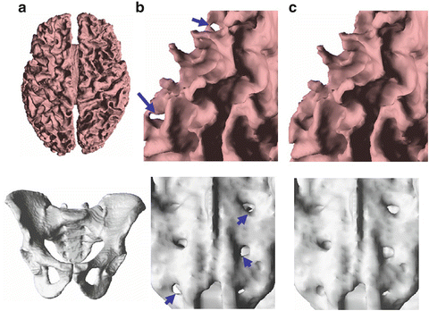

Fig. 2
Topologically-constrained segmentations. (a) shows the reconstructed surface; (b) shows close-up views of the standard GDM results; and (c) shows close-up views of the TGDM results
2.3 Shape Priors
Segmentation algorithms that only make use of low-level image information (such as intensity gradients) often fail to produce satisfactory results in medical imaging applications due to image noise, limited image resolution and contrast, and other imaging artifacts that often present in typical medical image data. In these cases, simple geometric regularization no longer suffices, and higher-level prior knowledge about the shape of desired object(s) can help.
The first published method that applies shape priors in GDM segmentation was proposed by Leventon et al. [57]. The method consists of two major stages. In the first stage, a statistical object shape model is computed from a set of training samples  , where each training shape
  is embedded as the zero level set of a signed distance function. Using principal component analysis (PCA), the covariance matrix of the training set is decomposed as
  , where U is a matrix whose column vectors represent the set of orthogonal modes of shape variation and Σ is a diagonal matrix of corresponding singular values. The first k columns of U form the eigenspace of the (typical) shapes. One can project a given shape Φ onto this shape space using
 where
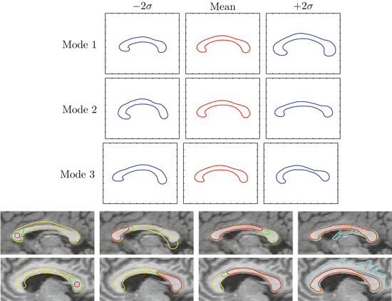
where  is the mean shape, and α is the k-dimensional vector of coefficients that represent Φ in the space spanned by U k . The shape model construction is illustrated in the top panel of Fig. 3. A training set of corpus callosa segmentation is analyzed by PCA and the three primary modes of variations of the shape distribution are shown in the figure. Assuming a Gaussian distribution for α, the probability of a new shape can be computed as:
 where Σ k contains the first k rows and columns of Σ.
 , where each training shape
  is embedded as the zero level set of a signed distance function. Using principal component analysis (PCA), the covariance matrix of the training set is decomposed as
  , where U is a matrix whose column vectors represent the set of orthogonal modes of shape variation and Σ is a diagonal matrix of corresponding singular values. The first k columns of U form the eigenspace of the (typical) shapes. One can project a given shape Φ onto this shape space using
 is the mean shape, and α is the k-dimensional vector of coefficients that represent Φ in the space spanned by U k . The shape model construction is illustrated in the top panel of Fig. 3. A training set of corpus callosa segmentation is analyzed by PCA and the three primary modes of variations of the shape distribution are shown in the figure. Assuming a Gaussian distribution for α, the probability of a new shape can be computed as:

Fig. 3
Top: The three primary modes of variations of the corpus callosum training data set. Bottom: Four steps in the segmentation of two different corpora callosa. The last image in each case shows the final segmentation in red. The cyan contour is the standard evolution without the shape influence. Image courtesy of the authors of [57]
In the second stage of the method, an active contour model is evolved both locally, based on image gradient and curvature information, and globally towards a maximum a posteriori (MAP) estimate of the shape and pose. At each iteration, the MAP estimates of the shape coefficients α ∗ and the pose parameter p ∗ are first computed, and the MAP estimate of the shape Φ ∗ is then determined. Incorporating the shape estimation into a traditional GAC model leads to a new level set evolution equation in the following form:
 The first two terms are the typical GAC model (as mentioned earlier) and the last term is the shape prior term. The parameter β is used to balance the influence of the shape model and the GAC model. The bottom panel of Fig. 3 compares the performance of the GAC model with and without using the shape prior. Due to weak edges, the GAC without the shape prior leaks out and fails to capture the desired shape; whereas the GAC with the proposed shape prior is well constrained and successfully converges to the boundary of the corpus callosum.

3 GDMs with Topology Control
Since the introduction of the original TGDM, several alternative approaches or extensions have been proposed in the literature. We briefly summarize these approaches in this section.
In the original TGDM, strict topology preservation is enforced, i.e., the number of connected components, cavities and handles are all constrained to remain unchanged [42]. Segonne et al. [92, 93] made the observation that TGDM can sometimes generate “topological barriers” that lead to geometric inconsistencies (cf. Fig. 4). They proposed to loosen the topological constraint so that only genus (i.e., the number of handles) is preserved. Their genus-preserving GDM (GGDM) allows connected components to merge, split, or vanish but no topological defects (i.e., handles) can be generated. To this end, the concept of “simple point” is extended to a“multisimple point” criterion, which is checked whenever the level set function is about to change sign at a computational point. Fig. 4 illustrates the benefit of the GGDM method.
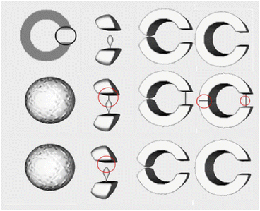

Fig. 4
Segmentation of a “C” shape using a spherical initialization. First row: GDM without topology control; second row: TGDM result; third row: GGDM result. Image courtesy of the authors of [93]
In both TGDM and GGDM, the topological constraint is enforced in the discrete sense. A few efforts have been made to formulate topology preservation in the continuous domain. Shi and Karl [97] proposed to use the so-called differentiable minimum shape distance (DMSD) to define a topological prior. DMSD is defined as the shortest distance between any two points on two closed curves. Cast in a variational framework, a topological prior term is introduced that is inversely proportional to the DMSD. The term approaches infinity when the DMSD between two curves approaches zero, thus preventing two curves from merging (though they can still split).
Alexandrov and Santosa [1] proposed a topology-preserving level set method for shape optimization. A topological constraint is built into the optimization problem by adding the following logarithmic barrier energy functional:
![$$\displaystyle{H(\varPhi ) = -\int _{\partial D}\log [\varPhi (\mathrm{x} + d\nabla \varPhi (\mathrm{x}))]\mathrm{d}s -\int _{\partial D}\log [-\varPhi (\mathrm{x} - l\nabla \varPhi (\mathrm{x}))]\mathrm{d}s}$$](/wp-content/uploads/2016/09/A151032_1_En_5_Chapter_Eque.gif) where Φ denotes the level set function,
where Φ denotes the level set function,  denotes the contour boundary, ds is the arc-length measure, and d > 0 and l > 0 are real numbers. These two terms probe in the vicinity of the contour boundary in the inner and outer normal directions, respectively, and penalize cases when points away from the zero level set have small absolute distance values. The energy functional has the effect similar to building “barriers” between merging or splitting contours, thus preventing such topological changes to happen.
![$$\displaystyle{H(\varPhi ) = -\int _{\partial D}\log [\varPhi (\mathrm{x} + d\nabla \varPhi (\mathrm{x}))]\mathrm{d}s -\int _{\partial D}\log [-\varPhi (\mathrm{x} - l\nabla \varPhi (\mathrm{x}))]\mathrm{d}s}$$](/wp-content/uploads/2016/09/A151032_1_En_5_Chapter_Eque.gif)
 denotes the contour boundary, ds is the arc-length measure, and d > 0 and l > 0 are real numbers. These two terms probe in the vicinity of the contour boundary in the inner and outer normal directions, respectively, and penalize cases when points away from the zero level set have small absolute distance values. The energy functional has the effect similar to building “barriers” between merging or splitting contours, thus preventing such topological changes to happen.
Sundaramoorthi and Yezzi [103] proposed to use a PDE-based geometric flow to achieve topology preservation. The flow minimizes the following energy functional:
 where C is a contour,
  and ds are the arc-length measures,
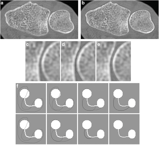
  is the Euclidean norm, and γ > 0 is a free parameter. Minimization of this energy functional leads to a repulsive force that prevents the model contour from self-intersecting or splitting. It also imposes a global regularization of the evolving contour. Fig. 5 demonstrates the benefit of this global regularizing force. Figs. 5(a)–(e) compare the segmentation results of TGDM and the global regularizing flow for a carpal bone image. Fig. 5(a) shows the contour initialization. Fig. 5(b) shows the final segmentation of the global regularization flow. A magnified view of the bone joint part is shown in Fig. 5(c), and the results of TGDM and the new method in this area are shown in Figs. 5(d) and (e), respectively. Clearly, the latter approach keeps the contours more separated. Fig. 5(f) is another demonstration using a toy problem. Since TGDM only uses a hard constraint that does not come into play until topology is about to change in the next step, it does not regularize the contour as the global regularizing flow does. A similar double integral energy was also used by Rochery et al. [83] for the extraction of a road network and by Guyader and Vese [40] who integrate this energy over regions and formulate it directly in the level set framework.

 and ds are the arc-length measures,
  is the Euclidean norm, and γ > 0 is a free parameter. Minimization of this energy functional leads to a repulsive force that prevents the model contour from self-intersecting or splitting. It also imposes a global regularization of the evolving contour. Fig. 5 demonstrates the benefit of this global regularizing force. Figs. 5(a)–(e) compare the segmentation results of TGDM and the global regularizing flow for a carpal bone image. Fig. 5(a) shows the contour initialization. Fig. 5(b) shows the final segmentation of the global regularization flow. A magnified view of the bone joint part is shown in Fig. 5(c), and the results of TGDM and the new method in this area are shown in Figs. 5(d) and (e), respectively. Clearly, the latter approach keeps the contours more separated. Fig. 5(f) is another demonstration using a toy problem. Since TGDM only uses a hard constraint that does not come into play until topology is about to change in the next step, it does not regularize the contour as the global regularizing flow does. A similar double integral energy was also used by Rochery et al. [83] for the extraction of a road network and by Guyader and Vese [40] who integrate this energy over regions and formulate it directly in the level set framework.
Fig. 5
(a)-(e): carpal bone segmentation. (f): a toy problem in which the “stuck” situation of TGDM is avoided by the global regularizing flow. (See text for details.) Image courtesy of the authors of [103]
4 GDMs Incorporating Shape Priors
Following the work of Leventon et al., many GDM methods that incorporate prior shape information have been recently proposed [24, 25, 87, 88, 107, 108, 124]. An extensive review can be found in [32]. We briefly summarize the major contributions.
Most of the shape-constrained GDM methods assume a linear model for shape variations, which tend to have two major limitations [21, 30, 31, 86]. First, the training shapes do not always satisfy a Gaussian distribution as typically assumed. Second, the space of signed distance functions is not linear, i.e. a linear combination of signed distance functions is in general no longer a signed distance function. To address these limitations, Cremers et al. [30, 31, 86] proposed a statistical shape prior based on an extension of classical kernel density estimators (cf. [81, 85]) to the level set domain. This prior statistically approximates an arbitrary distribution of training shapes (without making the restrictive assumption of a Gaussian distribution). In the limit of infinite sample size, the distribution inferred by the kernel density estimator converges towards a distribution on the manifold of signed distance functions. In addition, the cited works also embed an intrinsic alignment in the energy function so that the shape prior is invariant to certain group transformations such as translation and scaling. Fig. 6 compares the segmentation result of using a kernel prior against the results of using a uniform prior, a linear prior, and a manual segmentation. It can be seen that in this example, the result of using a kernel prior is closest to the manual segmentation.


Fig. 6
Comparison of the segmentations obtained with the kernel prior (white) and with alternative approaches (black). Image courtesy of the authors of [86]
Another development in shape prior modeling is the incorporation of object dynamics. In applications such as cardiac segmentation and tracking, it is important to take into account temporal correlations of the images. Cremers et al. [29] proposed to extend the shape modeling to learn the temporal dynamics of a deforming shape for the segmentation of an image sequence. The dynamical statistical shape model is constructed by approximating the shape vectors of a sequence of silhouettes by a Markov chain, which is then integrated into a Bayesian segmentation framework. Kohlberger et al. [54] proposed to treat time as an ordinary fourth dimension and applied a 4D PCA analysis on the training sequences to derive a 4D shape model. In this method, a whole volume sequence is segmented at the same time as a 4D image.
5 Fast GDMs
Since GDMs represent the model contour(s) using a higher-dimensional level set function, a heavy computational cost can be incurred with a naive implementation. To improve computational efficiency, narrowband methods in conjunction with reinitialization techniques [82, 95] are widely used to restrict the computation to the neighborhood of the evolving contour(s). However, the overall computation load can still be prohibitive when the grid size is large.
Several fast implementations of GDMs have been proposed. Goldenberg et al. [38] and Weickert et al. [113] proposed to adapt the additive operator splitting (AOS) scheme [114] for GDMs, which relaxes the stability constraint on the size of the time step associated with the explicit numerical schemes. The AOS scheme is very stable; but when large time steps are used, splitting artifacts may arise due to reduced rotational invariance. Kenigsberg et al. [48] and Papandreou and Maragos [77] proposed to use multigrid techniques to address this problem and to allow the use of even larger time steps than the AOS scheme. When sub-voxel accuracy is not of concern, Shi and Karl [96]’s method can provide a very high efficiency since it eliminates the need to solve the level set PDE. The method directly tests an optimality condition for the final curve location based on the speed functions, and uses only simple operations like insertion and deletion on two lists of boundary points to evolve the curve.
The reinitialization of the level set function can also be accelerated or even omitted. Krissian and Westin [56] proposed a fast implementation of the Chamfer distance to save computation time while maintaining the sub-voxel accuracy of the interface. Li et al. [58, 59] proposed a distance-preserving energy function that forces the level set function to be close to a signed distance function, which eliminates the need for re-initialization and improves the overall efficiency. Another distance-preserving level set method was later proposed by Estellers et al. [35]; it is more efficient due to the use of a splitting strategy and advanced  optimization techniques.
 optimization techniques.
Several new methods, constituting a new variational model for image segmentation that is closely related to the GDM, have been recently proposed [13, 19, 39]. These methods represent objects by soft membership functions rather than signed distance functions and the smoothness of the segmentation results is controlled by total variation regularization. The resulting models are convex and thus global optimal solutions can be guaranteed to be found. Also, the development of efficient convex relaxation methods [13, 39] allows such models to be computed much faster than traditional GDMs. One weakness, however, is that geometric properties of objects such as surface curvature and distances between coupled surfaces cannot be easily modeled and there is no control of the final segmentation topology. Such models have also been extended to the segmentation of multiple objects (cf. [6, 60]).
6 Adaptive Grid GDMs
The development of adaptive grid GDMs was motivated by the observation that the resolution of a GDM is directly limited by the resolution of the computational grid. One can improve the model resolution by using highly refined grids at the cost of losing efficiency and increasing the size—i.e., number of vertices—of the resulting contour(s). A more elegant approach to address the resolution and efficiency tradeoff is to use adaptive grid techniques [53], which locally refine or deform a coarse grid to concentrate computational efforts where more accuracy is needed. Incorporation of topological constraints also becomes feasible. Two types of adaptive grids have been used: the moving grid and the quadtree/octree grid. We briefly summarize these two types of approaches in the following.
A 2D moving grid GDM method was introduced in [41]; it maintains a fixed reference grid, but moves the actual physical grid points according to the desired image features [15, 63]. The adaptively deformed grid is obtained by first solving a Poisson equation using a DCT solver, and then solving an ordinary differential equation. After that, the level set PDE is solved on the deformed grid with narrow-banding. Since a uniform reference grid is always kept, the topology preserving principle on uniform grids (cf. Sect. 2.2) can be directly applied, by performing the simple point check directly on the reference grid.
An octree grid in 3D (or similarly a quadtree grid in 2D) is a hierarchical cartesian grid that is locally refined in regions of interest. These adaptive grids are widely used to improve accuracy in the solution of PDE’s [74, 104] and in medical image segmentation [8, 34, 122]. The cost for generating an adaptive octree grid is much smaller compared to that for a moving grid, since no partial differential equations need to be solved.
Implementation of topological constraints as introduced in TGDM is challenging, however, since the theories of common digital topology on uniform grids cannot be directly applied to an octree grid. Bai et al. [7, 8] proposed a new digital topology framework on octree grids that include new definitions of neighborhood, connectivities, and simple points. Based on this extension, a new octree-grid TGDM (OTGDM) method was introduced in [8, 9]. Adaptive octree grids are generated according to boundary curvature estimates, and the OTGDMs preserve the surface topology while evolving on octree grids.
A comparison is shown in Fig. 7 for the use of TGDM to extract inner and outer cortical surfaces from a brain image on three types of grids: a coarse uniform computational grid (of the original image size); a fine uniform computational grid (double size of the original image); and an octree grid whose finest grid resolution is same as the fine uniform grid. Figs. 7(a)–(c) show close-up views of the three inner surface results. It can be seen that the OTGDM result provides an adaptive multi-resolution representation of the surface mesh, which has large triangles in regions that are relatively flat and small triangles in regions with high curvatures. Figs. 7(d)–(g) show close-up cross-sectional views of the inner and outer surface results and the octree grids generated. It can be observed that the fine grid TGDM result and the OTGDM result capture anatomical details (such as the deeply folded sulci and gyri indicated by the circles) better than the coarse grid TGDM result.
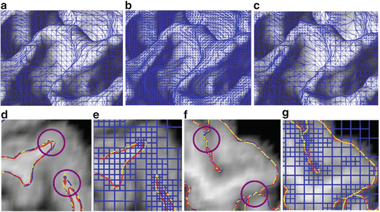

Fig. 7


Extraction of inner and outer surfaces using three computational grids. (a)–(c) triangle meshes: (a) coarse uniform grid TGDM result; (b) fine uniform grid TGDM result; (c) OTGDM result. (d) and (f): close-up views of inner and outer surfaces reconstructed by three types of grid: red–coarse uniform grid TGDM result, blue–fine uniform grid TGDM result, yellow–OTGDM result; (e) and (g): close-up views of octree grids used by OTGDM (shown in blue)
Stay updated, free articles. Join our Telegram channel

Full access? Get Clinical Tree


