Fig. 1
Schematic of the abdominal area of the human body showing the location of a the kidney
Fig. 2
A schematic showing the anatomy of the human kidney
The actual process of creating the urine from the blood takes place in the nephrons. Each nephron consists of a glomerulus, its tubule and its blood supply as seen in Fig. 3. The tubule is also divided into four parts: Bowman’s capsule, proximal tubule, loop of Henle, and distal tubule. The blood meets the glomerulus structure and the urine starts to formulate through three main processes. These processes include filtration by the glomerulus, as well as reabsorption and secretion by the tubular cells. By means of these processes, the important products such as the amino acids and water in the body are conserved, whereas the metabolic wastes (urea, uric acid, creatinine, ammonia) are excreted out of the body.
The first process, the filtration, occurs in the glomerulus. The differences in the blood pressure and the protein osmotic (oncotic) pressure allow the glomerulus to act as an ultra-filter and allow only small particles to enter the fluid that goes into the Bowman’s capsule. As a result, the fluid enters the Bowman’s capsule lacks the blood cells and the proteins. From the Bowman’s capsule, this filtrated fluid goes into the tubular cells which actively transport the necessary materials such as glucose back into the body. This active transportation is called reabsorption, and it helps to retain normal blood levels of necessary materials. On the other hand, a process called secretion is responsible for removing some substances from the blood and adding to the tubular [33]. By the end of these three steps, the urine of a healthy kidney should be free of protein, glucose, and any blood cells.
Fig. 3
Structure of a nephron
In ultrasound, ultrasonic sound waves are transferred at high frequency by a transducer, and transfer through the skin and other body tissues to the kidney. The sound waves reflect from the kidney like an echo and come back to the transducer. The transducer collects the reflected waves, which are then altered into an electronic image of the kidney. The speed at which the waves travel is highly affected by various types of body tissues. By introducing additional mode to the ultrasound, the blood flow could be estimated. A Doppler probe inside the transducer gauges the velocity and direction of blood flow in the vessel by allowing sound waves to be audible. The loudness degree of the sound waves shows the level of blood flow in a blood vessel. Also, obstruction of blood flow could be determined by the absence of these sounds. In DCE-MRI, as the contrast agent Gd-DTPA passes through the cortex, the signal intensity is expected to increase before it decreases slightly due to water reabsorption. Constant signal intensity is then expected followed by a decrease due to the washout of the contrast agent. In a healthy kidney, the signal intensity increases instantly after the contrast agent is introduced in around 40 s and peaks within 100 s and starts to drop slowly to its initial value while the urine is formed [34].
Ultrasound
Ultrasound is currently still the first choice in the early assessment of the transplanted kidney or in the long-term follow-up. After 24–48 h posttransplantation, a baseline US evaluation is performed with a detailed examination of renal size, echogenicity, collecting system, ureter condition, and evaluation of any postoperative collections. Graft enlargement (swelling, more globular shape), reduction of corticomedullary differentiation, increased echogenicity, prominent medullary pyramids, or irregularities in the graft perfusion are all typical US findings in case of acute renal rejection [12]. Color Doppler (CD) and power Doppler (PD) are used to investigate blood flow in the renal and iliac vessels, and “flow quantification” can be measured using resistivity index (RI), pulsatility index (PI), and systolic/diastolic ratio [22]. The Doppler resistive index (RI) developed by Leandre Pourcelot is a measure of pulsatile blood flow that mirrors the resistance to blood flow caused by microvascular bed distal to the site of measurement. RI is usually determined as a standard practice in clinical monitoring, and it can depend on the recipient’s vessels and their elasticity beside the graft vessels [35]. RI was found to be a useful parameter in quantifying the variations in renal blood flow that might be associated with renal disease. RI is defined as  , where PSV: peak systolic velocity and EDV: end diastolic velocity [36]. Figure 4 shows how RI is calculated from a CD sonogram. Contrast-enhanced Ultrasound (CEUS) is used to evaluate cortical perfusion since CD and PD can only estimate perfusion in large arteries [37], see Fig. 5.
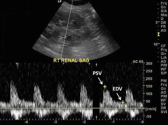
, where PSV: peak systolic velocity and EDV: end diastolic velocity [36]. Figure 4 shows how RI is calculated from a CD sonogram. Contrast-enhanced Ultrasound (CEUS) is used to evaluate cortical perfusion since CD and PD can only estimate perfusion in large arteries [37], see Fig. 5.Fig. 4
The process of calculating renal resistance index from CD sonogram
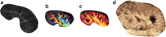
Fig. 5
Illustration of gray-scale sonography (a), color Doppler (b), power Doppler (c), and CEUS (d). Note that CD or PD cannot evaluate the cortical perfusion; however, CEUS can explore this area
Recently, the are several studies that evaluate the performance of the conventional ultrasound parameters such as the resistance index (RI) in the diagnosis of early allograft dysfunction. According to [38, 39], RI is not an exact indicator of renal graft dysfunction, and it could only provide a prognostic marker of the graft. Saracino et al. [40] concluded that RI measurements taken early after kidney transplant could predict long-term renal function. However, Kramann et al. [23] focused in their research on evaluating the ability of RI measurements to predict renal allograft survival on the time point of RI measurement. They found that RI measurements should be taken 12–18 months posttranplantation in order to be able to predict long-term allograft survival. Also, Khosroshahi et al. [41] compared Doppler US images of the donor’s kidney before and 6–12 months after transplantation and showed that a significant increase in the RI couldn’t be related to the graft enlargement. Krejčí et al. [42] examined the potential of US evaluation in the detection of subclinical acute rejection using a composite gray-scale, CD, and PD imaging, and it was proven that a significant differentiation between different groups could be achieved. Damasio et al. [43] investigated the use of Doppler US in the case of dual kidney transplantation (DKT), and it was concluded that DKT patients had higher RI and lower kidney volumes than single kidney transplantation (SKT) patients. Chudek et al. [44] tried to characterize factors that influence PI and RI in patients with immediate (IGF), slow (SGF), or delayed (DGF) kidney graft function, and found that ischemic injury which occurred mainly prior to organ harvesting played a dominant role determining intrarenal resistance in the early posttransplant period. Fischer et al. [45] proved the superiority of ultrasound contrast media (USCM) to conventional US that uses the RI indicator in the diagnosis of early allograft dysfunction. In addition, Benozzi et al. [46] found that both US and CEUS could identify grafts with early dysfunction, but only some CEUS-derived parameters could differentiate between ATN and acute renal rejection. A summary of recent studies relating to acute renal rejection with different US findings is given in Table 1.
Table 1
Summary of studies on acute renal rejection with different US findings
Study | Objective | Methods | Conclusions |
|---|---|---|---|
Fischer et al. [45] | Compare the ability of USCM in diagnosing early allograft dysfunction with the traditional US modalities that relies on the RI parameter. | An overall of 48 successive kidney recipients undertook US examination after USCM administration 4–10 days after transplantation. | Conventional US that rely on RI measurements are inferior to USCM when it comes to diagnosing early kidney allograft dysfunction. |
Kirkpantur et al. [38] | Investigate the correlation relationship between RI and renal histopathologic characteristics in grafted kidneys. | The intrarenal RI was retrospectively compared with biopsy results in 28 kidney recipients. | RI appeared to offer a predictive indicator for the graft rather than yielding a precise diagnosis of renal graft dysfunction. |
Kramann et al. [23] | Evaluate the ability of RI measurements to predict renal allograft survival through a retrospective single-center analysis, but with special focus on the time point of RI measurement. | In total, 88 patients with an RI measurement 0−3, 3−6, and 12−18 months after transplantation were involved and separated into two groups according to RI threshold of 0.75. | RI obtained 12−18 months after transplantation was found to be able to help in predicting long-term allograft results, while RI acquired during the first 6 months after transplantation failed to predict renal allograft dysfunction. |
Seiler et al. [39] | Test the hypothesis that renal RI represents a sign of systemic vascular damage rather than an organ-specific indicator. | Renal and splenic RIs besides common carotid intima-media thickness (IMT) were measured in 87 stable transplant recipients. | Results backed the belief that renal RI is not a specific marker of allograft dysfunction. |
Benozzi et al. [46] | Compare the results of CEUS and PD in renal transplanted kidneys within 30 days after transplantation. | Altogether, 39 kidney recipients experienced CEUS and US examinations at 5, 15, and 30 days after transplantation. The outcomes were correlated with clinical findings and functional evolution. | Although US and CEUS both could recognize grafts with early dysfunction, only some CEUS-derived factors could separate ATN from acute renal rejection. |
Krejčí et al. [42] | Assess the prospect of ultrasound evaluation in the recognition of subclinical acute rejection that are diagnosed in stable grafts by protocol biopsy. | Gray-scale assessment, CD imaging, and PD imaging were performed before each of 184 protocol graft biopsies in 77 patients in the third week, third month, and first year after transplantation. | Groups with borderline changes and subclinical acute rejection and groups with normal histological finding and clinically manifested acute rejection could be successfully divided using a combined gray-scale, PD and CD assessment. |
Damasio et al. [43] | Analyze CD results in patients with dual kidney transplantation (DKT) and compare renal volume and resistive index (RI) values between DKT and single kidney transplantation (SKT). | Reviewing the clinical and imaging findings [30 CDUS, five magnetic resonance (MR) and one computed tomography (CT) examination] in 30 patients with DKT. Renal volumes and RI were compared with 14 SKT patients and comparable levels of renal function. | CD provided beneficial information in patients with DKT, and DKT patients had higher RI and lower volumes than SKT patients. |
Khosroshahi et al. [41] | Compare the Doppler US variations in the donor’s kidney before transplantation with the recipient’s kidney at 6 to 12 months after transplantation. | Before transplantation, the size, cortical thickness, echogenicity, anastomosis, mean pulsatility index (MPI), and RI of the 20 kidney donors were documented. In addition, the same parameters were measured in the recipient’s kidney at 6 to 12 months after transplantation | Findings showed a significant enlargement of the kidney size accompanied with an insignificant increase in MPI and RI of the transplanted kidney. |
Saracino et al. [40] | Evaluate the potential for RI measured early after kidney transplant to also predict long-term renal function. | RI measurements of 79 transplant patients within 1 month after the transplant were divided into two groups based on RI median value of 0.635. | Early determination of RI can help predict long-term graft function in kidney transplant recipients. |
Chudek et al. [44] | Describe factors that affect PI and RI in patients with immediate (IGF), slow (SGF), or delayed (DGF) kidney graft function. | PI and RI were measured in 200 transplanted patients at 2 to 4 days after transplantation. Patients with acute rejection episodes within the first month were discarded. IGF, SGF, and DGF were defined based on different creatinine levels. | A central role in the determination of intrarenal resistance in the early period after transplantation is played by ischemic injury, which transpired primarily prior to organ harvesting. |
Magnetic Resonance Imaging
Magnetic resonance imaging (MRI) has become the most powerful and central noninvasive tool for clinical diagnosis of diseases [47]. The main advantage of MRI is that it offers the best soft tissue contrast among all imaging modalities (e.g., US and CT). However, structural MRI lacks functional information. Dynamic contrast-enhanced magnetic resonance imaging (DCE-MRI) is a special MR technique that has emerged as a new noninvasive technique to provide superior information of the anatomy, function, and metabolism of tissue [26, 48]. The technique involves the acquisition of serial MR images with high temporal resolution before, during, and several times after the administration of a contrast agent (e.g., gadolinium) into the blood stream. In DCE-MRI, the signal intensity in target tissue changes in proportion to the contrast agent concentration in the volume element of measurement, or voxel. DCE-MRI is commonly used to enhance the contrast between different tissues, particularly normal and pathological. A typical example of a dynamic MRI time series data of the kidney is shown in Fig. 6.
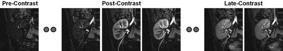
Fig. 6
DCE-MRI images taken at different time points post the adminstration of the contrast agent showing the change of the contrast as the contrast agent perfuses into the tissue beds for kidney
DCE-MRI has been extensively used in many clinical applications, including the study of the hemodynamic (i.e., perfusion) and properties of tissues (blood flow, blood volume, mean transit time), microvascular permeability and extracellular leakage space, detection of renal transplant diseases, and MR angiography [49]. Advantages of DCE-MRI techniques over other imaging modalities include the lack of ionizing radiation, increased spatial resolution, the ability to provide superior anatomical and functional information, and the feasibility to be used as early as possible (even one day posttransplantation) for the assessment and follow-up of the transplanted kidney. Unlike the brain where the widely used clinical agent gadolinium is confined by the blood–brain barrier and behaves essentially like an intravascular agent, in the kidney tissue the contrast agent gadolinium behaves as a leakage agent, namely it distributes in the extra cellular extra vascular space, and at short times (up to about 2 min) after administration at DCE-MRI, time-intensity curves (TIC) that represent the average intensity of the kidney can be constructed. Importantly, from these TICs empirical parameters (indexes) that reflect the delivery of agent to the tissue bed can be estimated (see Fig. 7). Other clinically important functional parameters, such as fractional plasma volume (FPV), renal blood flow (RBF), glomerular filtration rate (GFR), renal plasma flow (RPF), and cortical and medullary blood volumes, can also be estimated from the perfusion curves [50]. Whereas these TICs represent global information about the kidney condition, it is conceivable that a vascular insult can be confined to a local territory. Thus for visual local assessment it is helpful for the radiologists that the perfusion indexes can be displayed as pixel-by-pixel parametric maps (see Fig. 8) overlayed on an anatomic image. This is of great importance, in case of kidney dysfunction, the radiologist can investigate which kidney regions need attention during follow-up of the treatment and thus determine the appropriate therapy.
Fig. 7
Typical DCE-MRI TIC representing the average intensity of the kidney measured before and after the adminstration of the contrast agent into the blood stream. The figure illustrates typical transient phase (peak value, time to the first peak, and the initial up-slope) and the tissue distribution phase parameters that can be estimated and used for diagnosis
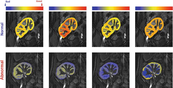
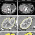
Fig. 8
Perfusion maps for the four perfusion indexes estimated from the normalized TICs: peak signal intensity (first column), initial up-slope (third column), average plateau (second column), and time-to-peak (last column); for a normal subject (upper row) and acute rejection subject (lower row). The red and blue hues of each color scale correspond to respective highest and lowest values, respectively. Note all indexes show worsening of perfusion with pathology
Developing a CAD for early and noninvasive diagnosis of the kidney is an ongoing area for research interest. However, DCE-MRI exhibits multiple challenges stemming from (1) the need to image very quickly, to capture the transient first-pass transit effects, while maintaining adequate spatial resolution (2) varying signal intensities over the time course of agent transit, and (3) nonrigid deformations, or shape changes, may occur related to pulsatile or transmitted effects from adjacent structures, such as bowel. A schematic diagram of a typical CAD system for detection of acute rejection is shown in Fig. 9. The motion correction step of the kidney on DCE-MRI time series is a preprocessing step in developing the CAD system to compensate for the global and/or local motion of the kidney. Next, the kidney objects are segmented and the functional unit (i.e., renal cortex) is extracted in order to determine dynamic agent delivery. In the final step, perfusion is estimated from contrast agent kinetics using empiric indexes (see Fig. 7) and classification is performed based on the extracted features to distinguish between acute rejection and non-rejection. Below, we will overview the related work on renal image segmentation and registration as well as the todays’ CAD systems for kidney diagnosis.
Fig. 9
Typical computer-aided diagnosis (CAD) system for diagnosis of acute renal rejection. The input of a CAD system is the DCE-MRI medical images. The motion correction step is used to handle global and/or local motion during data acquisition. The renal cortex is segmented after kidney object segmentation since it is the cortex that is primarily affected by the perfusion deficits that underlie the pathophysiology of acute rejection. Then, the time intensity curves are constructed and perfusion features are extracted and used for diagnosis
Related Work on Renal Image Segmentation and Registration
Dynamic MR images are subject to relatively low signal-to-noise, nonuniform intensity distribution over the time series images, and geometric kidney deformations caused by gross patient motion, transmitted respiratory effects, and intrinsic and transmitted pulsatile effects. Therefore, accurate segmentation and registration of dynamic MR renal images is a challenge. These two basic steps are commanding the major attention in this research area for automated analysis of dynamic perfusion MRI. Particularly, kidney motion effects can be compensated for by specific use of global and local registration techniques. On the other hand, kidney segmentation techniques can be classified into three main categories: threshold-based, deformable boundary-based, and probabilistic or energy minimization-based methods. Below we review the related work on kidney segmentation and registration techniques addressing the above-mentioned challenges.
Threshold-based techniques segment the kidney and its internal structures (i.e., cortex and medulla) by analyzing an empirical probability distribution, or histogram of pixel intensities in a region-of-interest (ROI). Earlier computerized renal image analysis (e.g., [51–54]) was usually carried out either manually or semiautomatically. Typically, the user defines an ROI in one image and for the rest of the images, image edges were detected and the model curve was matched to these edges. However, the manual ROI placements are based on the users’ knowledge of anatomy and thus are subject to inter- and intra-observer variability. Also, valuable information, being inherent in the DCE-MRI signal intensity time series (sequences), is not used. Additionally, these approaches are very slow, even though semiautomated techniques (e.g., [51, 54]) do reduce the processing time. Giele et al. [55] introduced an approach for the segmentation and registration and of the kidney on DCE-MRI. First, the kidney contour is drawn manually by the user in a single high-contrast image. Then, the phase difference movement detection (PDMD) method is employed to correct kidney displacements. Their method demonstrated better performance than direct image intensity matching and cross-correlation. However, when compared with the radiologist results, the PDMD method accuracy was about 68 % and a manual mask to register the time frames was still required. Additionally, only translational motion was handled, while rotational motion was not mentioned, although the existence of the latter has been discussed in a number of studies [51, 56, 57]. De Priester et al. [54] subtracted the average of pre-contrasted images (10 frames) from the average of early enhanced images (30 frames) and thresholded the resulting difference image to obtain a kidney mask. Objects smaller than a certain size (700 pixels) were removed, and the remaining kidney object was closed using morphological erosion and manual processing. This approach was further expanded by Giele [58] by applying an erosion filter to the mask image in order to obtain a contour at a second subtraction stage. Koh et al.[59] segmented kidneys with the morphological 3D H-maxima transform. Rectangular masks and edge information are used to exclude training data or prior knowledge. Simple thresholding is too inaccurate to segment human organs in DCE-MRI, because these specific regions have similar gray level (intensity) distributions.
Evolving deformable boundary methods have been explored as a more accurate means of kidney segmentation. A series of studies on both rats and human subjects [57, 60–65] has been conducted for the registration and segmentation of kidneys from DCE-MRI. A multi-step segmentation and registration in the study on humans by Sun et al. [57, 62] initially corrects the large-scale motion by using an image gradient-based similarity rigid registration (only translational). Once roughly aligned, a high-contrast image is subtracted from a pre-contrast image and a level set approach was used to extract the kidney border from the difference image. Then, the segmented kidney contour is propagated over the other frames to search for the rigid (rotation and translation) registration parameters. For rat studies, Sun et al. [60, 61, 63] used a variational level set approach to find the kidney borders. Their framework integrated a subpixel motion model and temporal smoothness constraints. For segmenting the cortex and medulla, the level set approach by Chan and Vese [66] was used. The deformable model-based segmentation has been improved by hybrid edge- and region-based models in a number of studies [67, 68]. Some works have focused on segmenting multiple objects with multiphase level set methods [69, 70]. Abdelmunim et al. [71] incorporated both image and shape prior information into a variational level set framework for kidney segmentation. However, their model did not adequately account for spatial dependencies between the pixels and therefore are quite sensitive to imperfect kidney contours and image noise. Yuksel et al. [72, 73] proposed a parametric deformable model approach for the segmentation of the kidney where the deformable contour evolution was constrained using two density functions. The first describes the kidney shape prior and is constructed using the average signed distance maps of the training samples. The second functional describes the pixel-wise image intensity distribution of the kidney and its background, estimated using an adaptive linear combinations of discrete Gaussians (LCDG) [74–81]. El-Baz et al. [82–84] proposed a parametric deformable model-based approach for the segmentation of the kidney using shape and visual appearance priors. The shape model is constructed from a linear combination of vectors of distances between the training boundaries and their common centroid. The appearance prior is modeled with a spatially homogeneous second-order Markov-Gibbs random field (MGRF) of gray levels with analytically estimated pairwise potentials. The current appearance model is described with the LCDG model [74–81]. Khalifa et al. [29, 85] proposed an automated level set-based framework for the segmentation of kidney from dynamic MRI. They proposed a stochastic force that accounts for a shape prior and features of image intensity and pairwise MGRF spatial interactions [75, 86–88]. These features are integrated into a joint MGRF image model of the kidney and its background to constrain the evolution of the deformable contour [89–92]. They employed a two-stage registration methodology using first an affine transformation to account for the global motion, followed by a partial differential equation (PDE)-based approach for local motion correction [90, 92]. The segmentation approach in [29, 89] was later extended to deal with 3D data in [93, 94]. Gloger et al. [95] presented a level set-based approach using the shape prior information and Bayesian statistical concepts for generating the shape probability maps. However, the shape prior model in [29, 89, 93–95] did not impose temporal constraints on kidney segmentation.
The graph cut-based segmentation algorithm by Boykov et al. [96, 97] minimizes the energy of a temporal MGRF model of intensity curves. Each voxel is described with a vector of intensity values over time. Initially, several seed points are placed on the objects and on the background to give user-defined constraints as well as expert samples of intensity curves. These samples are used to compute a two-dimensional histogram further acting as a data penalty function in minimizing the energy. Although the results looked promising, manual interaction was still required. Rusinek et al. [98] proposed a graph cut-based segmentation formwork to assess cortical and medullary functional parameters. Their method employed a rigid registration step to account for the kidney displacements and the approach has been tested on simulated and in-vivo data. Ali et al. [99] used the graph cut-based minimization of an energy functional combining a shape constraint with boundary properties. The constraint was built using a Poisson probability distribution and distance maps. Chevaillier et al. [100, 101] proposed a semiautomated method to segment internal structures (i.e., cortex, medulla, and pelvis) from DCE-MRI time series by using k-means-based partitioning to classify pixels according to contrast evolution using vector quantization algorithm. However, it was only tested on eight data sets for normal kidneys, and user interaction was still required. A similar segmentation by Song et al. [102] has only been tested on two MRI data sets, with simulated rotation and translation rigid motion, for one normal and one abnormal kidney. An automated framework proposed by Zöllner et al. [103] assesses renal function by deriving voxel-based functional information from DCE-MRI, the nonrigid image registration compensating for the motion and deformation of the kidney during DCE-MRI acquisitions. The k-means clustering method [104] was used for extracting functional information about different regions of the kidney according to their dynamic contrast enhancement patterns. An automated wavelet-based k-means clustering framework for segmenting the kidneys was proposed by Li et al. [105]. The images were co-aligned using B-splines registration and cross-correlation (CC) cost function and their framework was tested on seven subjects (four volunteers and three patients). Yang et al. [106] proposed a framework for the classification of kidney tissue using fuzzy c-mean clustering. In order to reduce the motion artifacts, their framework employed a nonrigid registration step using the demons algorithm [107] and the squared pixel distance as a similarity metric and the squared gradient of the transformation field as the smoothness regularization term. To summarize, the reviewed methodologies for kidney segmentation and registration are presented in Table 2.
Table 2
Summary of kidney segmentation and registration techniques using MRI
Study | Database | Dim | AL | Approach | Performance |
|---|---|---|---|---|---|
De Priester et al. [54] | 18 data sets (9 subjects) | 2D | UI | • Thresholding, • Morphological erosion and manual processing. | N/A |
5 data sets | 2D | UI | • Manual segmentation of the kidney, • PDMD registration. | ACC: 68 % | |
Sun et al. [62] | 5 subjects | 2D | UI | • Multi-step rigid registration, • level set segmentation for the kidney and the cortex. | Error is at most one pixel size (for one sequence of 150 image frames) |
20 data sets | 2D | A | • Variational level set. | Visual evaluation by an expert. | |
Abdelmunim et al. [71] | 39 data sets to build shape prior (Testing data N/A) | 2D | A | • Shape-based segmentation using level set. | N/A |
N/A | 2D | UI | • Shape-based segmentation using parametric deformable model. | E: 0.382 % (for one image only) | |
2700 images | 2D | A | • Scale invariant feature transform (SIFT)-based alignment, • Shape-based segmentation using parametric deformable model, • Second-order MGRF spatial interaction model of gray scale images. | E: 0.83±0.45 % | |
Khalifa et al. [29] | 26 data sets | 2D | A | • Affine registration, • Shape-based segmentation using level set, • Second-order MGRF spatial interaction model. | E: 1.29±0.60 |
Khalifa et al. [85] | 50 data sets | 2D | A | • Affine registration, • Shape-based segmentation using level set, • Higher-order MGRF spatial interaction model. | DSC: 0.982±0.016 |
Khalifa et al. [127] | 50 data sets | 2D | A | • Affine registration, • Shape-based segmentation using level set, • Second-order MGRF spatial interaction model. | DSC: 0.970±0.02 |
Boykov et al. [96] | 18 data sets |