Fig. 1
A colon reconstructed from its (a) supine and (b) prone scans
In this paper, we present a method of supine-prone registration using conformal colon flattening. Conformal colon flattening has been introduced as an enhancement for VC navigation [14] and has been utilized successfully for CAD [5]. According to conformal geometry theory, there exists an angle preserving map which periodically flattens the colon surface onto a planar rectangle. This mapping minimizes the total stretching energy. Because the conformal mapping is locally shape preserving, it offers an effective way to visualize the entire colon surface and exposes all of the geometric structures hidden in the original shape embedded in 3D.
The characteristics of the deformation between supine and prone are determined by the elasticity properties of the tissues and muscles. The strain-stress relations for different types of tissues or muscles are different. If the strain-stress relation deformation is independent of the orientation, then local deformation is practically a scaling, and the global deformation is conformal. In that case, we can flatten each supine and prone surface to a planar rectangle conformally, and those two rectangles should be similar. By aligning the planar rectangles, we can get a one-to-one and onto mapping and obtain the registration between them. In this work, we introduce this registration approach and carefully design experiments to test whether the deformation between supine and prone is conformal or not. Our experimental results show that the deformation is not conformal, but close to conformal.
An elastic deformation with bounded angle distortion is called a quasi-conformal map. The angle distortion for a quasi-conformal map can be represented as a complex valued function, the so-called Beltrami coefficient. The Beltrami coefficient fully controls the quasi-conformal map, which is determined by the elasticity of the underlying material. By better understanding the deformation between supine and prone, we can understand the elasticity of the tissues and muscles and vice versa.
The nonrigid elastic deformation between supine and prone colons poses a great challenge for shape registration. In this work, we locate and match the anatomical landmarks [15], including flexures and taeniae coli, and internal features on conformally flattened supine and prone surfaces [16], and compute the registration by harmonic maps with these feature constraints. The resulting supine-prone registration is a quasi-conformal map (diffeomorphism), which reflects the elastic deformation of the muscle and tissue. The distortion is evaluated by the Beltrami coefficients. Our experiments on 6 pairs of supine-prone colons obtained an average ℝ 3 distance error of 7.85 mm for the feature points and polyps evaluated. To the best of our knowledge, this is the first work to apply geometric mapping for supine-prone colon registration by converting the 3D registration problem to a 2D image matching problem. The whole process is efficient and automatic, and our registration method performs better than other existing methods (see section “Analytic Registration Evaluation”).
Fig. 2
The pipeline for supine-prone colon registration
Figure 2 shows our registration pipeline, which primarily consists of five stages. As the input, the supine and prone CT scans are subjected to the pre-processing steps, including cleansing, segmentation with topological simplification, and surface mesh reconstruction, which have been studied previously and are outside the scope of this paper. Given the supine and prone surfaces, anatomical landmarks are extracted (see section “Taeniae Coli and Flexures Extraction” and [15]). Using these landmarks, the colon surfaces of both supine and prone are decomposed to segments. For each segment, a flat rectangular conformal mapping is obtained (see section “Conformal Colon Flattening”). Based on these flat images, feature points are detected and their correspondences between supine and prone are obtained (see [15]). With the feature correspondence constraints, the supine-prone registration is performed using harmonic maps (see sections “Quasi-Conformal Map” and “Surface Registration Framework”).
Given the completed supine-prone registration, we present the methods in which we visualize the results of our registration algorithm. We first demonstrate flattened rendering of the colon in the native 2D registration format (see section “Flattened Colon Rendering”). For the endoluminal views which would be used by a radiologist reading a case, we detail a method to provide correlated views between supine and prone (see section “Visualization of Quasi-Conformality”). To better understand where the deformation occurs most on the colon surface, we show the visualization of the Beltrami coefficient both in 2D and 3D (see section “Visualization of Quasi-Conformality”). The results of our registration are analyzed and discussed in section “Experimental Results”. We verify the efficacy of our work using both objective analytic and subjective visual methods. We present the related work in the next section and brief background information on conformal mapping and quasi-conformal mapping in section “Conformal Geometry Theory” to familiarize the reader with the terms.
Related Work
Early work on supine-prone registration for VC applications focused on using the centerlines and various landmarks. A basic method applies linear stretching and shrinking operations to the centerline, where local extrema are matched and used to drive the deformations [11]. Improved methods of centerline correlation were also investigated for use in reducing false positive results [13]. Correlating individual points along the centerline through the use of dynamic programming has also been suggested [12, 17].
More recently, the taeniae coli (three bands of smooth muscle along the colon surface) have been used as features which can be correlated between the two scans [18, 19]. This relies on a manual identification of one of the three taeniae coli, and then an automatic algorithm repeats the line representing the identified taenia coli at equal distances. Further progress has been made where the haustral folds and the points between them can be automatically detected, and the taeniae coli are identified by connecting these points [20]. However, this method is only feasible on the ascending and transverse portions of the colon.
Deformation fields have also been suggested for use in supine-prone registration. Motion vectors can be identified for matched centerline regions, interpolated for non-matched regions, and then propagated to the entire volume [21]. It has also been proposed to use a free-form deformation grid to model the possible changes in the colon shape from supine to prone [22].
Conformal mapping has been successfully used for many medical applications, such as brain cortex surface morphology study [23] and colonic polyp detection [5]. In this work, we perform the supine-prone registration through conformal mapping based on Ricci flow. The colon surface is reconstructed from CT images, represented as a topological cylinder in the discrete form of a triangular mesh, and conformally mapped to a planar rectangle. The subsequent registration is carried out through the 2D conformal mapping images of the supine and prone colons.
Ricci flow was first introduced by Hamilton [24] and later it was generalized to the discrete case [25]. Ricci flow is a powerful tool to compute surface uniformization, deforming any arbitrary surfaces to one of the 3 canonical spaces with different background geometries, the sphere, the Euclidean plane, or the hyperbolic disk. The discrete computational algorithms can be found in [26–29]. Ricci flow can also be generalized to compute general quasi-conformal maps by the auxiliary metric method [30]. Discrete surface Ricci flow method has been successfully used in many applications in both engineering and medical imaging, such as general 3D shape matching, registration and tracking [27, 31, 32], shape indexing and comparison in Teichmüller space [33], homotopy detection [29], vestibular system morphometry [34], brain mapping [35, 36], 3D human facial expression recognition [37], virtual colonoscopy [16, 38], wireless sensor network routing, load balancing and data storage [39–42], and so on.
Because the deformation from supine to prone is not conformal, we generalize the conformal colon flattening method to a quasi-conformal flattening for registration purpose. Most existing colon registration methods cannot guarantee the mapping to be a diffeomorphism (one-to-one and onto mapping). Due to the complicated geometric structure of the colon surface, the existing methods often introduce folding or singularities in the mapping. Our method is based on the biophysical nature of the deformation from supine to prone, which is physically elastic and anisotropic. Due to the material properties of the muscles and tissues, the deformation can be exactly modeled as a quasi-conformal map. Our experimental results validate that the mapping is indeed quasi-conformal.
Conformal Geometry Theory
This section briefly introduces the background knowledge in conformal geometry, necessary for the discussion in the work. For more details, we refer readers to [43] for Riemann surface theory, [44] for Teichmüller theory, [45] for quasi-conformal mapping, and [46] for differential geometry.
Conformal Mapping
Let S 1, S 2 be two metric surfaces, with Riemannian metrics g 1 and g 2, respectively. A map φ : S 1 → S 2 is angle-preserving or conformal, if and only if the pull back metric induced by ϕ satisfies
 where e 2λ is called the conformal factor. The simplest conformal mapping is the complex holomorphic functions f : ℂ → ℂ, satisfying the Cauchy–Riemann equation
 where
where  and the complex differential operators are
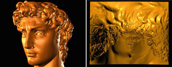
and the complex differential operators areFig. 3
Conformal mapping preserves local shapes
Locally, a conformal mapping is a scaling transformation; therefore, it preserves local shapes. As shown in Fig. 3, the 3D surface of Michelangelo’s David head is conformally mapped to the planar rectangle, although the global shape has been distorted, the local shapes are well preserved. On the planar image, one can still easily locate the main geometric features. This property is valuable for virtual colonoscopy, where the colon wall surface is conformally flattened onto a 2D image. Because the mapping is shape-preserving, the polyps can be detected on the planar image directly.
Given an oriented metric surface (S,g), U ⊂ S is a neighborhood, then there is a conformal mapping φ from the unit disk  to U, such that the Riemannian metric is written in a special form
 where
where  are called isothermal parameters of the surface. Suppose the surface is covered by an atlas, such that all local coordinates are isothermal parameters, and all the chart transitions are biholomorphic, then the atlas is called a conformal structure of the surface, induced by the Riemannian metric. A surface with a conformal structure is called a Riemann surface.
to U, such that the Riemannian metric is written in a special form are called isothermal parameters of the surface. Suppose the surface is covered by an atlas, such that all local coordinates are isothermal parameters, and all the chart transitions are biholomorphic, then the atlas is called a conformal structure of the surface, induced by the Riemannian metric. A surface with a conformal structure is called a Riemann surface.Uniformization
Fig. 4
Uniformization for surfaces, computed by discrete surface Ricci flow
The surface uniformization theorem claims that for any metric surface (S,g), there exists a unique conformal factor e 2λ, such that the Riemannian metric e 2λ g induces a constant Gaussian curvature, which is one three possible choices  depending on the surface topology.
depending on the surface topology.As shown in Fig. 4, for closed surfaces, genus zero surfaces can conformally mapped to the unit sphere  , genus one surfaces can conformally deformed to Euclidean metric
  , high genus surfaces can conformally deformed to hyperbolic metric ℍ 2. For compact surfaces with boundaries, all the boundaries are mapped to circles on the canonical domains, as shown in the right half of the figure.
, genus one surfaces can conformally deformed to Euclidean metric , high genus surfaces can conformally deformed to hyperbolic metric ℍ 2. For compact surfaces with boundaries, all the boundaries are mapped to circles on the canonical domains, as shown in the right half of the figure.The uniformization theorem allows us to map all types of shapes to one of the three canonical domains, the sphere, the plane, or the hyperbolic disk and register the shapes on the 2D canonical domain. This simplifies the problem of surface matching and registration and has been broadly applied in medical imaging field.
Quasi-Conformal Mapping
Fig. 5
Comparison between conformal mapping (frame 2 and 3) and a general diffeomorphism (frame 4 and 5)
Figure 5 shows another characteristic of conformal mappings, it maps infinitesimal circles to infinitesimal circles. In contrast, a general diffeomorphism maps infinitesimal circles to infinitesimal ellipses. The general diffeomorphisms are represented as quasi-conformal map.
Given two Riemann surfaces S 1 and S 2 with conformal atlases, choose a local conformal parameter (isothermal parameters) z for S 1 and w for S 2, respectively. Let f : S → D is a diffeomorphism between the surfaces, then its local representation is w = f(z), the Beltrami coefficient of the mapping f is defined as
(1)
Globally, one can use Beltrami differential  to represent the mapping. At each point z, the eccentricity and the orientation of the infinitesimal ellipse are given by
 as shown in Fig. 6.
to represent the mapping. At each point z, the eccentricity and the orientation of the infinitesimal ellipse are given byFig. 6
Geometric interpretation of Beltrami coefficient
General diffeomorphisms between surfaces (induced by natural deformations) are quasi-conformal mappings. Each quasi-conformal mapping is associated with its Beltrami differential. Inversely, the mapping can be uniquely determined by its Beltrami differential (under certain normalization conditions) by solving the so-called Beltrami equation,
(2)
For example, consider all the normalized diffeomorphisms from the unit disk to itself,  , such that f(0) = 0 and f(1) = 1, then the space of normalized diffeomorphisms and the space of Beltrami coefficients have a one-to-one correspondence.

, such that f(0) = 0 and f(1) = 1, then the space of normalized diffeomorphisms and the space of Beltrami coefficients have a one-to-one correspondence.Suppose (S 1,g 1) and (S 2,g 2) are two metric surfaces, with local isothermal parameters z and w, respectively. φ : (S 1,g 1) → (S 2,g 2) is a quasi-conformal mapping with Beltrami coefficient μ. Then the same mapping  under the auxiliary metric
is conformal. Therefore a quasi-conformal mapping can be converted to be a conformal mapping under the auxiliary metric associated with the Beltrami coefficient.
under the auxiliary metric(3)
Surface Ricci Flow
Surface Ricci flow is a powerful tool to design Riemannian metrics using prescribed Gaussian curvatures, it can be applied for computing surface conformal mappings and quasi-conformal mappings directly.
Let both g and  are Riemannian metrics of a surface S,
  , then the Gaussian curvature and geodesic curvature induced by them satisfies the following Yamabe equation:
are Riemannian metrics of a surface S, , then the Gaussian curvature and geodesic curvature induced by them satisfies the following Yamabe equation:The surface uniformization metric can be obtained by solving the Yamabe equation. Surface Ricci flow is an effective tool for it.
The normalized surface Ricci flow is given as
 where ρ is the mean value of the scalar curvature
 where A(0) is the total area of the surface at time t = 0, χ(S) is the Euler characteristic number of the surface. It can be shown that the normalized surface Ricci flow preserves the total area
 furthermore, the curvature evolves according to a nonlinear heat diffusion process
Harmonic Mapping
Suppose φ : (S 1,g 1) → (S 2,g 2) is a smooth mapping between two metric surfaces. We choose isothermal parameters of the two surfaces, z for S 1 and w for S 2, respectively, the Riemannian metrics can be represented as
The harmonic energy of the mapping is defined as
(4)
The so-called harmonic maps are the minimizers of the harmonic energy. The necessary condition of φ to be a harmonic is the Euler–Lagrange equation
Given a degree one map, we can use the following nonlinear heat diffusion method to deform it to a harmonic map,
(5)
From the Definition 4, we see the harmonic energy is solely determined by the conformal structure of the source and the Riemannian metric of the target. One can deform the conformal structure by a Beltrami differential μ, then obtain the conformal coordinates ζ(z), which can be obtained by solving the Beltrami equation.
Harmonic map is the smoothest map in the homotopy class (Fig. 7). If the surfaces are topological disks, the restriction of φ on the boundary is a homeomorphism, then the harmonic map is a diffeomorphism. Furthermore, if the target surface has Riemannian metric with negative Gaussian curvature, then degree one harmonic map must be a diffeomorphism. Harmonic maps have been applied for brain mapping and colon registration in medical imaging.
Computational Strategies
There are many methods for conformal surface mapping in the literature. In the following, we focus on the discrete surface Ricci flow method.
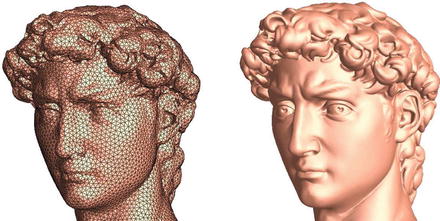
Fig. 8
Smooth surfaces are approximated by triangle meshes
Discrete Surface Ricci Flow
In practice, surfaces are represented as simplicial complex, namely triangle mesh as shown in Fig. 8. We use M = (V,E,F) to denote the mesh with vertex set V , edge set E, and face set F. A discrete Riemannian metric on a triangle mesh is a function defined on the edges, l : E → ℝ +, satisfies triangular inequality, on each face [v i ,v j ,v k ],
 where α i ’s are corner angles adjacent to the vertex v, ∂ M represents the boundary of the mesh (Fig. 9).
Fig. 9
Discrete curvatures
Then the discrete curvatures also satisfy Gauss–Bonnet theorem, namely, the total curvature is a topological invariant
Surface Ricci flow conformally deforms the Riemannian metric, conformal transformation preserves infinitesimal circles. Thurston proposes to replace infinitesimal circles to circles with finite sizes, and by changing the circle radii to approximate the conformal deformation.
Fig. 10
Configurations
Figure 10 shows the common configurations. For the first frame, which is classical Thurston’s circle packing, a circle is centered at each vertex v i , and denoted as (v i ,γ i ), two circles at the end vertices of an edge [v i ,v j ] has an intersection angle ϕ i j , during the deformation, ϕ i j keeps unchanged. The edge length
The second frame shows the inversive distance circle packing, where two circles at an edge are disjoint, the edge length is given by
 where I i j is called the inversive distance, which is a constant during Ricci flow. The third frame shows the discrete Yamabe flow, where

The last frame shows the circle packing with imaginary radius, the edge length is given by
The power circle is the circle orthogonal to all the three circles centered at the vertices. In Yamabe flow case, the power circle is the circum circle of the triangle; in the case of circle packing with imaginary radius, the power circle is the equator of a hemisphere, which goes through the points (x i ,y i ,γ i 2), where v i = (x i ,y i ). The center of the power circle is called the power center. The lines through the power center perpendicular to edge [v i ,v j ] separates the edge to d i j and d j i
 Approach to Detection and Characterization of Hepatic Hemangiomas
 Resonance Imaging of Adenocarcinoma of the Pancreas
 Imaging of the Liver
 Self-Parameterized Active Contours for Medical Image Segmentation with Emphasis on Abdomen
 Imaging with VHF Signal Generation: A New Contrast Mechanism for Cancer Imaging Over Large Fields of View
 Liver Segmentation Without Prior Statistical Models


Related posts:
Approach to Detection and Characterization of Hepatic Hemangiomas
Resonance Imaging of Adenocarcinoma of the Pancreas
Imaging of the Liver
Self-Parameterized Active Contours for Medical Image Segmentation with Emphasis on Abdomen
Liver Segmentation Without Prior Statistical Models
Stay updated, free articles. Join our Telegram channel
Full access? Get Clinical Tree
