Algorithm 1: The model-free segmentation approach
Input: Contrast enhanced CT volume and the set of fixed parameters.
Output: Binary volume, liver is the foreground.
Procedure:
Step-1: Performing image normalization in soft tissue window and then applying nonlinear diffusion filter to each slice.
Step-2: Selecting one slice as the start slice and then define the liver landmarks on it.
Step-3: Estimating initial shape, intensity, and graph cuts constrains from the start slice.
for all lower slices, starting from the start slice to the last one. do
Step-4: Define a narrow band around the liver object.
Step-5: Performing slice segmentation using shape-based graph cuts algorithm.
Step-6: Adding the segmentation results of this slice to the output volume.
Step-7: Updating shape, intensity, and graph cuts constrains according to current slice segmentation.
end for
for all upper slices, starting from the start slice to the first one. do
Repeat Step-4 and Step-5.
if the segmented object contains multiple parts then
Step-8: Selecting the left most one as the liver object.
end if
Repeat Step-6 and Step-7.
end for
Step-9: Applying the post-processing procedure to the output volume.
return output volume.
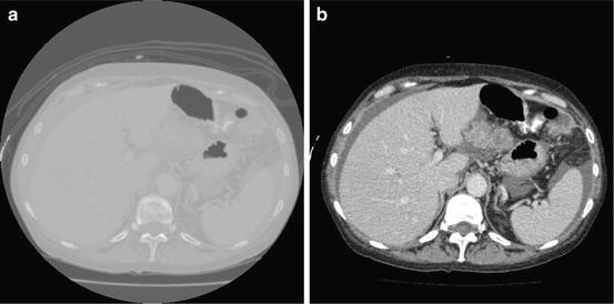
This window is determined by plotting the histogram of the raw data and selecting the lower and upper bounds of the right distribution in the histogram as shown in Fig. 1. Then, these lower and upper bounds are used to map the original raw data to a grayscale data according to (1). The original image and the produced gray scale one are shown in Fig. 2:
where I o is the raw CT image, I g is the produced gray level image, Lo is the selected lower intensity bound, and Hi is the selected upper intensity bound.
(1)
Fig. 1
Determination of the lower and upper bounds used for intensity mapping
Fig. 2
Mapping the raw CT data to grayscale image, (a) original data, and (b) the produced gray image
After mapping the whole CT volume to a grayscale volume, a nonlinear diffusion filter [42, 43] is applied to each 2D slice in the volume to reduce the noise and to increase the liver homogeneity. In contrast to the convolution and rank filters (median filter, mean filter, etc.), the nonlinear diffusion filter can remove the noise from homogenous areas while keeping clear and sharp edges as shown in Fig. 3. The nonlinear diffusion filter is obtained by the time solution of (2):
where I g (x,y,0) is the original gray image, t refers to the iteration steps, and C is a diffusivity function that depends on the gradient magnitude of the image.  is a smoothed version of I(x,y) which is obtained by convolving it with a Gaussian of standard deviation σ g . In this work, a rapidly decreasing diffusivity function suggested in [44] is implemented as
![$$ C=\left\{\begin{array}{ccc}\hfill 1\hfill & \hfill \mathrm{if}\hfill & \hfill g\le 0\hfill \\ {}\hfill 1-{\mathrm{e}}^{-\frac{3.315}{{\left(g/K\right)}^4}}\hfill & \hfill \mathrm{if}\hfill & \hfill g>0\hfill \end{array}\right.. $$” src=”/wp-content/uploads/2016/03/A303895_1_En_11_Chapter_Equ3.gif”></DIV></DIV><br />
<DIV class=EquationNumber>(3)</DIV></DIV></DIV><br />
<DIV class=Para>The conductance parameter, <SPAN class=EmphasisTypeItalic>K</SPAN>, determines the contrast of edges that will have significant effect on the smoothing.</DIV><br />
<DIV></DIV><br />
<DIV id=Sec4 class=]()
(2)
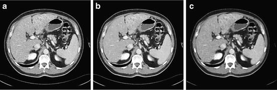
is a smoothed version of I(x,y) which is obtained by convolving it with a Gaussian of standard deviation σ g . In this work, a rapidly decreasing diffusivity function suggested in [44] is implemented asFig. 3
Output of the preprocessing step, (a) input image, (b) smoothed image using a nonlinear diffusion filter, and (c) smoothed image using the median filter
Initialization
A simple user interaction is required to determine and segment one slice in the CT volume. The segmentation result of this slice, represented as a binary template, is used to define the initial shape constrains as well as the initial intensity model of the corresponding case. Consequently, these constrains are automatically propagated in a slice-by-slice manner.
From the anatomical knowledge of the liver, we can divide the whole CT volume into two main parts: the upper part and the lower part. In the upper part, the liver starts as a single small object behind the heart, and it grows up to be a single large object at the end of this part. In the lower part, the liver starts as a single large object, and it is divided into two or more segments and then ends as a single small object behind the colon and the kidney as shown in Fig. 4. These two parts are separated by a slice containing nearly the largest cross section of the liver, which is selected as the starting slice for segmentation. In this slice, the liver object is very clear and its boundary can be distinguished from the other objects visually. Therefore, the initial liver segmentation is performed in less than 1 min according to the following procedure:
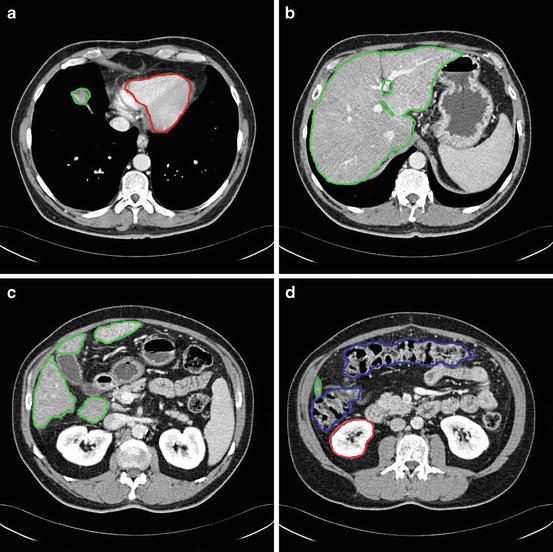
Fig. 4
The main anatomical structure of the liver, (a) start slice of the liver (liver in green and cardiac in red), (b) end of the upper part, (c) a slice in the lower part with a liver divided to four segments, and (d) the end slice of the liver (liver in green, kidney in red, and colon in blue)
1.
The user selects from 20 to 30 landmarks on the liver boundary as shown in Fig. 5a.
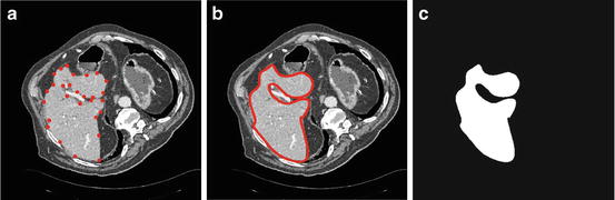
Fig. 5
Start slice segmentation, (a) selected landmarks, (b) estimated liver boundary, and (c) corresponding shape template
2.
Estimation of the Shape and Intensity Constrains
The shape constrains are applied as a prior probability of the liver location, and the intensity constrains are defined as the probability of the liver intensity model at each pixel. These constrains are automatically determined for each slice according to the segmented liver object in the previous slice. The estimation process is performed according to the following procedure:
1.
Define the binary liver template in the start slice as Temp str , the binary liver object in this slice as object str , the binary liver template in the previous slice as Temp prv , the binary liver object in this slice as object prv , the pixels belonging to the liver in the previous slice as Liver prv , and the pixels not belonging to the liver in the previous slice as non ‐ Liver prv .
2.
Determine the minor axis of the ellipse that fit the object in Temp prv and denote it as m ax (Fig. 6a).
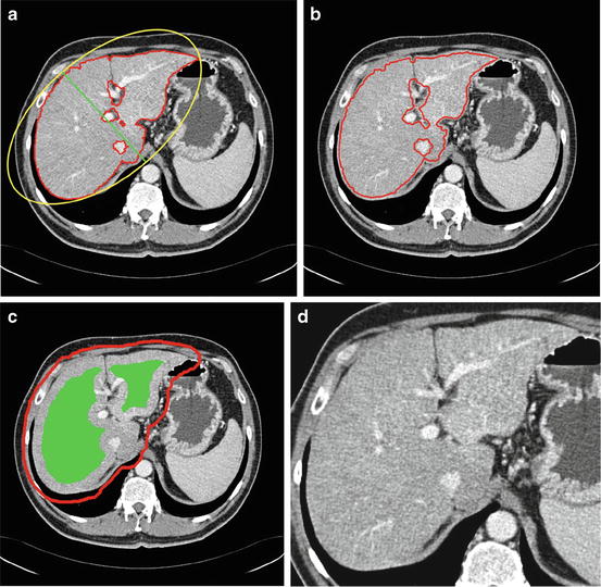
Fig. 6
Constrain estimation, (a) sample previous slice (liver contour in red and the minor axis in green), (b) the contour of the estimated shape template shown on the current slice, (c) the estimated constrains for graph cut (object in green and background in red), and (d) the slice after applying the narrow band constrain
3.
Erode the Temp prv with a disk structuring element of radius round(0.02 × m ax ) and consider the result as the shape template of the current slice (Fig. 6b). This erosion value has been decided after studying the average change of the minor liver axes in different cases.
4.
If Area(object prv ) ≥ 0.1 × Area(object str ), calculate the histogram of Liver prv and non ‐ Liver prv as the intensity model; else, use the previously used intensity model.
5.
Erode Temp prv with a disk structuring element of radius round(0.1 × m ax ) and the result is considered as the object hard constrains in the graph cut algorithm (Fig. 6c).
6.
Dilate the Temp prv with a disk structuring element of radius max(2, round(0.1 × m ax )). Then, the edge of the resulting binary template is determined and dilated with a disk structuring element of radius 1. The result of this step is considered as the background hard constrains in the graph cut algorithm (Fig. 6c).
7.
Define a narrow band window surrounding the liver object as the smallest rectangle fitting the dilated object calculated in step 5 (Fig. 6d).
Segmentation Using Graph Cuts
Introduction to Graph Cuts
An image segmentation problem can be considered as a binary labeling problem. In which, a unique label A p ∈ “obj”, “bkg” is assigned to each pixel in the image. A good labeling or segmentation A, A = A 1, A 2, …, A |P| : |P| is the number of image pixel, has to minimize a predefined energy function. Boykov et al. [46] introduced a solution for this problem using a graph cut algorithm. In the graph cuts, a graph G = 〈V, ε〉 is defined as a set of nodes V and a set of edges ε. The nodes of the graph represent the image pixels in addition to two specially designated terminal nodes S (source) and T (sink), which represent the object and background labels. The set of edges ε in the graph includes two types of edges: edges between neighboring pixels, which are defined as n-links, and edges connecting all pixels to the terminal nodes, which are defined as t-links. All graph edges e ∈ ε, including n-links and t-links, are assigned some nonnegative weight/cost w e . An example of a simple 2D graph of 3 × 3 image is shown in Fig. 7a.
Fig. 7
An undirected graph of 3 × 3 image (a) and (b) s − t cut. The thickness of the edges represents their costs. Figure based on [41]
A binary label A p that partition the underlying image into object and background segments can be obtained by determining an s − t cut on the graph. The s − t cut is a subset of edges C ∈ ε such that the terminals S and T become completely separated by removing these edges as shown in Fig. 7b. The cost of a cut is defined as the sum of the weights/costs of all edges included in that cut, |C| = ∑ e ∈ C w e . The cut with a minimal cost gives the optimal segmentation according to the designated energy function. It is important to formulate a precise energy function that can be encoded via n-links and t-links. In addition, a set of hard constrains for object and background, similar to these introduced in [47], can be imposed using infinity cost t-links. The graph cut algorithm has been successfully applied to liver vessels segmentation in [48] and to interactive 2D and 3D images segmentation in [49–52].
The goal of energy minimization is to find a labeling A = {A 1, A 2, …, A |p|}, which minimize the Gibbs energy function E(A) defined in (4):
where

and
(4)
(5)
(6)
(7)
The parameter μ in (4) determines the relative importance of the boundary term, B(A), versus the regional term, R(A), and ℵ p defines the neighborhood of pixel p. R p (A p ) is the penalty of assigning a label A p to a pixel p, and B pq (A p ,A q ) is the penalty of labeling the pair of pixels p and q with labels A p and A q , respectively. In the presented approach, this energy function is adjusted to include the shape constrains as a penalty added to the regional term. Hence, the regional term R(A) is computed by adding two penalties: the data penalty R D (A p ) and the shape penalty R s (A p ). The data penalty reflects on how the intensity of pixel p fits into the intensity model of the object (liver) and background (non-liver tissues). The shape penalty is encoded as the prior probability of a pixel to be inside or outside the liver object. The data, shape, and boundary penalties are calculated as in (8), (9), and (10), respectively:
where shape temp is the estimated shape template of the objected (liver) in the current slice, I p is the intensity value of a pixel p, pr(I p ∈ ” obj ” (” bkg “)) is the probability of p to be an object (” obj “) or background (” bkg “) pixel, and d(p,q) is the Euclidian distance between pixels p and q. The total energy function can be obtained by including the shape penalty into the Gibbs energy function as shown in (11):

(8)
(9)
(10)
(11)
The parameter λ determines the relative importance of the data penalty versus the shape penalty. This total energy function can be minimized efficiently using the graph cut algorithm. To achieve this goal, a graph with cut cost equaling the value of E T (A) is constructed using the edge weights defined in (12), (13), and (14). Furthermore, the hard constrains defined in section “Estimation of the Shape and Intensity Constrains” are implemented via infinity cost edges:
(12)
(13)
(14)
Post-processing
In this stage, any tissue surrounded completely by the segmented liver tissue is added to the final segmentation, which smoothed using a 3D filter. To achieve this goal, the following procedure is applied:
1.
Perform a hole filling to each 2D slice.
2.
Perform binary image closing to the 3D volume using a ball-structuring element of radius 3.
3.
Perform a hole filling to each 2D slice again.
4.
Smooth the final volume by applying a binary median filter of 3 × 3 × 3 size.
Data and Experimental Setup
In this work, we perform a qualitative evaluation of the model-free segmentation approach using three datasets: both training and testing datasets of MICCAI2007 [53] and JAMIT contest dataset [54]. In this section, data description, evaluation metrics, and the parameter setting of the introduced segmentation approach will be introduced.
Datasets
The first dataset used for evaluation is the MICCAI2007 training dataset. This dataset contains 20 CT images acquired using a variety of CT scanners, including 4, 16, and 64 detector rows. All of these images were acquired contrast-dye-enhanced in the central venous phase. According to the machine and protocol used, pixel spacing is varied from 0.55 to 0.8 mm in x/y direction, and the slice spacing is varied from 1 to 5 mm. In some cases, the entire anatomy is rotated around the z-axes. Most images in this dataset have liver abnormalities, including tumors, metastasis, and cysts of different sizes. The second dataset is the MICCAI2007 testing dataset, which contains 10 CT images and has the same characteristic of the previous dataset. The third dataset is the dataset used in JAMIT contest for liver tumor detection. This dataset contains 20 CT images acquired contrast-dye-enhanced in portal venous phase. The pixel spacing is varied from 0.5 to 1 mm in x/y direction, and the slice spacing is varied from 0.8 to 1 mm. This data is used at the contest for liver tumor detection, and it has different kinds of liver abnormalities, including tumors and cysts.
Parameter Setting
The number of iteration of the nonlinear diffusion filter influences the quality of the smoothing process and then affects the homogeneity of the liver. A large number of iterations make the object more smooth; however, it greatly increases the processing time. From numerous experiments on randomly selected cases from MICCAI2007 training dataset, we set the number of iterations to 10. This value is optimal for keeping the balance between the object smoothing and the processing time. The other parameters of the nonlinear diffusion filter, time step, and K were set to 0.125, 1.5, and 3, respectively. Graph cut parameters have been adjusted using 5 CT images having different characteristics: 3 from MICCAI2007 training dataset and 2 from JAMIT dataset. Parameter μ, which determines the influence of the boundary penalty, was set to 2. The parameter λ, which determines the influence of the shape penalty in the regional term, was set to 0.2. These parameters were fixed for all images in all datasets. The parameter σ in the boundary term was dynamically selected from each slice as the average absolute intensity difference between the neighboring pixels (15):
(15)
Evaluation Metrics
(16)
(17)
(18)
(19)
(20)
Evaluation was performed using two sets of evaluation metrics. The first set of metrics contains five general segmentation metrics of sensitivity (16), specificity (17), precision (18), accuracy (19), and the error rate (20).
The second set of metrics, which was used in MICCAI2007 Grand Challenge workshop [55], includes five metrics. Two of these metrics are volume based and the other three are surface based. These five metrics are calculated for a segmented liver volume A and a reference liver volume B as the following:
1.
Volumetric overlap error (VOE), in percent: it is 0 for a perfect segmentation and 100 if the two volumes A and B do not overlap at all:
(21)
2.
Relative volume difference (RVD), in percent: a positive value refers to over-segmentation and a negative value refers to under-segmentation. The value of 0 means that both A and B have the same volume; however, it does not imply that they are identical [55]:
(22)
3.
Average symmetric surface distance (ASD), in mm: the value of 0 refers to a perfect segmentation: for each surface voxel of A, the Euclidian distance from the closest surface voxel of B is calculated. This distance is also calculated from B to A. The ASD is computed as the average of these distances.
4.
Root mean square symmetric surface distance (RMD), in mm: it is similar to the ASD; however, instead of Euclidian distance, the squared distance is calculated. The RMD is computed as the square root of the average squared distance.
5.
Maximum symmetric surface distance (MSD), in mm: it is similar to ASD; however, instead of the average, the maximal Euclidian distance is calculated.
Heimann et al. [55] provide a methodology for combining these different measures in one precision score. They transform the result ρ i of each error measure i to a gauged score φ i ∈ [0,100] and the final score is then computed as the average of all scores. To perform this transformation, they use a manual segmentation of non-expert to get the average user errors ρ′ i for each measure. Considering the performance of the manual segmentation as 75 out of 100, they calculate the corresponding score for measure i as
(23)
The score of 100 points represents a perfect segmentation, and a score of 75 can be regarded as equivalent to non-expert segmentation. They also reported that the error measures of the non-expert are equivalent to 6.4 %, 4.7 %, 1, 1.8, and 19 mm for VOD, the absolute value of RVD, ASD, RMD, and MSD, respectively.
Results
The segmentation approach was applied to 50 CT images described in section “Datasets.” We implemented the approach using Matlab® environment on Windows®-based personal computer with a Corei7 (2.8 GHz) processor and 6GB of memory. In order to reduce the processing time required for the smoothing stage, it was performed in parallel on the eight cores of the Corei7 processor using the Matlab® parallel computing toolbox.
Experiments on Clinical Data
The shape constrains play an essential role in the introduced model-free segmentation approach. The estimation of these constrains from the adjacent slice is assessed by computing the Jaccard coefficient (24), between the estimated shape and the manually segmented liver object at each slice. Figure 8 shows the computed coefficient between the true liver object and the estimated shape template and between the true liver object and the segmented one. From this figure, we can prove that the estimated template provides a good knowledge about the position and the shape of the true liver objects at each slice even in the case of large slice spacing:
(24)
where L is the estimated shape template and M is the manually segmented object.
Fig. 8
The Jaccard coefficient between the true liver object and the estimated shape template in blue, and the coefficient between the true liver objected and the segmented one in red: (a) sample from the MICCAI2007 training dataset with slice spacing of 1 mm, (b) sample from the MICCAI2007 training dataset with slice spacing of 5 mm, and (c) sample from JAMIT dataset with slice spacing of 1 mm
The evaluation results of the proposed approach using the first set of metrics are shown in Table 1 for the MICCAI2007 training dataset and in Table 2 for the JAMIT dataset. The evaluation of the MICCAI2007 testing dataset using this set of metrics is not available because the ground truth of this dataset is not publicly available.
Table 1
Evaluation of the results for the MICCAI2007 training dataset based on general segmentation metrics
Case | Sensitivity | Specificity | Precision | Accuracy | Error rate % |
|---|---|---|---|---|---|
#1 | 0.9790 | 0.9971 | 0.9467 | 0.9962 | 0.3799 |
#2 | 0.9815 | 0.9940 | 0.9472 | 0.9927 | 0.7282 |
#3 | 0.9838 | 0.9966 | 0.9472 | 0.9958 | 0.4177 |
#4 | 0.9686 | 0.9983 | 0.9698 | 0.9967 | 0.3266 |
#5 | 0.9803 | 0.9988 | 0.9732 | 0.9981 | 0.1922 |
#6 | 0.9854 | 0.9973 | 0.9486 | 0.9968 | 0.3235 |
#7 | 0.9318 | 0.9993 | 0.9832 | 0.9964 | 0.3581 |
#8 | 0.9436 | 0.9972 | 0.9686 | 0.9928 | 0.7187 |
#9 | 0.9583 | 0.9991 | 0.9828 | 0.9969 | 0.3095 |
#10 | 0.9754 | 0.9963 | 0.9560 | 0.9947 | 0.5290 |
#11 | 0.9849 | 0.9985 | 0.9715 | 0.9978 | 0.2224 |
#12 | 0.9855 | 0.9980 | 0.9645 | 0.9973 | 0.2694 |
#13 | 0.9434 | 0.9984 | 0.9693 | 0.9957 | 0.4310 |
#14 | 0.9788 | 0.9992 | 0.9677 | 0.9987 | 0.1263 |
#15 | 0.9806 | 0.9993 | 0.9793 | 0.9987 | 0.1334 |
#16 | 0.9715 | 0.9966 | 0.9662 | 0.9942 | 0.5758 |
#17 | 0.9840 | 0.9976 | 0.9559 | 0.9970 | 0.3030 |
#18 | 0.9707 | 0.9972 | 0.9495 | 0.9959 | 0.4134 |
#19 | 0.9655 | 0.9973 | 0.9628 | 0.9952 | 0.4828 |
#20 | 0.9618 | 0.9986 | 0.9551 | 0.9975 | 0.2490 |
Average | 0.9707 | 0.9977 | 0.9633 | 0.9963 | 0.3745 |
Std. dev. | 0.0157 | 0.0013 | 0.0119 | 0.0017 |