Dynamic Susceptibility Contrast MRI: Technical Considerations and Practical Issues

Fernando Calamante, PhD

▪ Introduction and Historical Background

Dynamic susceptibility contrast (DSC) MRI is an imaging technique that can be used to measure blood flow and other related hemodynamic parameters. It involves the intravenous injection of a paramagnetic MR contrast agent and relies on measuring and modeling the induced changes in T₂ and T₂★ relaxation, brought about by the induced susceptibility effect (Fig. 7.1). These changes are amplified when the contrast agent remains compartmentalized¹: the compartmentalization of the contrast agent leads to magnetic field perturbations that extend beyond the vascular space, thus creating long-range distortions to the magnetic field. These field inhomogeneities induce dephasing and therefore a shortening of T₂ and T₂★.¹ Due to this amplified effect related to compartmentalization, DSC-MRI is a technique that has primarily been used to assess cerebral perfusion: the blood vessels in the brain are surrounded by the so-called blood-brain barrier (BBB), which, when intact, makes the gadolinium-based contrast agents commonly used for DSC-MRI behave effectively as an intravascular contrast agent.^a This chapter will therefore solely focus in DSC-MRI as a brain imaging tool.

From a historical point of view, DSC-MRI was first described by Arno Villringer, Bruce Rosen, and colleagues at Massachusetts General Hospital in the late 1980s,¹ using fast one-dimensional data in rat brains. This pioneering work was quickly followed by further imaging studies in dog and human brains, and the potential major clinical role of this technique was quickly recognized, with several major advances carried out in those early years,²,³,⁴,⁵ and ⁶ which provided a very strong foundation for what this technique has now grown into.

Within the field of perfusion MRI, the terms cerebral perfusion, perfusion, cerebral blood flow, and its acronym CBF are all used indistinguishably. This same convention will be adopted throughout this chapter. Cerebral perfusion is arguably one of the key physiologic parameters in the brain, because it plays a central role to ensure tissue viability and function. Cerebral perfusion is responsible for the delivery of oxygen and nutrients and for the removal of waste products. It is therefore not surprising that numerous disease processes involve in one way or another disturbances to blood flow supply and that the development of robust methods to measure perfusion has been a major area of research in neuroimaging.

Some of the major attractions of DSC-MRI lie in its simple acquisition method [typically a single-shot echo-planar imaging (EPI) sequence], its short acquisition time (approximately 1 min), relative high signal-to-noise ratio (SNR) compared with other perfusion imaging methods (e.g., perfusion CT, arterial spin labeling, PET) (Fig. 7.2), and the wealth of information that can be obtained from the same acquired data set.

In the following sections, we will discuss the issues related to setting up a DSC-MRI protocol (both from the contrast agent, as well as from the MRI sequence points of view), introduce the concept of the arterial input function (AIF) and why its measurement is essential for CBF quantification, and describe the kinetic model used in DSC-MRI quantification and the role of the convolution and deconvolution mathematical steps. This will be followed by a description of the various parameters that can be calculated from DSC-MRI data, the practical factors to take into account to achieve quantification in absolute units, as well as the main technical limitations and errors that users must be aware of, including the modifications to the acquisition and analysis pipeline in order to deal with the presence of contrast agent extravasation (i.e., with BBB leakage). Finally, we will end the chapter with a brief description of the summary steps involved in a typical DSC-MRI study as well as a discussion regarding the current trend toward the use of fully automatic (black box) tools in DSC-MRI.

▪ Contrast Agent and the DSC-MRI Protocol

Despite being a perfusion imaging method that involves no ionizing radiation (and therefore often referred to as a noninvasive perfusion imaging technique), DSC-MRI does require the bolus injection of an exogenous MR contrast agent. This bolus, typically injected in the antecubital vein,⁷ most often involves a gadoliniumchelated contrast agent.⁴

The contrast dose, usually indicated as mL or mmol per kilogram of body weight, must be sufficient to induce a robustly measured transient signal drop (Fig. 7.1), and its optimal value depends on several factors such as the magnetic field strength, sequence parameters, injection rate, and type of contrast agent. In general,
for a typical acquisition protocol at 3 T using one of the standard 0.5 M concentration contrast agents, a so-called single dose (equivalent to 0.1 mmol/kg or 0.2 mL/kg) is recommended.⁷

Figure 7-1. Effect of a bolus of contrast agent in the signal intensity data from a patient with right internal carotid artery stenosis (left side of the images). Top row: Eight images acquired during the first passage of the bolus through the brain; the number under each image indicates the image number (corresponding to the shaded time interval in the graph). Bottom row: Signal intensity time course for a contralateral region of interest (see insert). The images and the time course clearly show the transient decrease in signal intensity introduced by the contrast agent. (Figure previously published in Calamante F. Perfusion MRI using dynamic-susceptibility contrast MRI: quantification issues in patient studies. Top Magn Reson Imaging 2010;21(2):75-85, reprinted with permission of Lippincott Williams & Wilkins, © 2011.)

It is now a common practice to inject this bolus of contrast agent by using an MR-compatible power injector. This contributes to ensure a well-defined bolus, with relative good consistency between studies. However, it is important to emphasize that, even for a perfectly controlled injection protocol (i.e., injection volume, site, and rate), the bolus shape entering the brain cannot be ensured to be reproducible and consistent; this shape is primarily dominated
by the passage of the bolus from the site of injection, through the heart-lungs-heart system, and then through the arterial vasculature to the brain. Therefore, other factors such as the cardiac output and arterial status can play a major role in determining the shape. This is one of the main reasons why the measurement of the AIF (see next section) is essential for CBF quantification.

Figure 7-2. Figure illustrating the larger contrast-to-noise ratio (CNR) of DSC-MRI (left column) than arterial spin labeling (ASL, middle column) and perfusion CT (pCT, right column). The plots in the bottom row show data for a typical volume of interest (VOI), in white matter, as highlighted by the square region in each image shown in the top row. The VOIs are 39, 54, and 150 µL for the DSC-MRI, ASL, and pCT cases, respectively. Note that despite the smaller volume for the DSC-MRI region, the CNR is much higher, where the transient drop with the arrival of the bolus can be readily appreciated. On the other hand, both ASL and pCT methods are very noisy in white matter regions, and the non-zero offset for ASL (dashed line) or the transient signal increase for pCT is much more difficult to detect. (Figure previously published in Calamante F. Arterial input function in perfusion MRI: a comprehensive review. Prog Nucl Magn Reson Spectrosc 2013;74:1-32, reprinted with permission of Elsevier, © 2013.)

Figure 7-3. Contrast agent concentration corresponding to the data shown in Fig. 7.1. Top row: Contrast concentration images for eight time points during the first passage of the bolus; the number under each image indicates the image number (see shaded time interval in the graph). Bottom row: Time-dependent concentration for a contralateral region of interest (see insert); due to the shape of the curve, these data are usually referred to as the “peak.” The data clearly show the transient increase in contrast agent concentration. (Figure previously published in Calamante F. Perfusion MRI using dynamic-susceptibility contrast MRI: quantification issues in patient studies. Top Magn Reson Imaging 2010;21(2):75-85, reprinted with permission of Lippincott Williams & Wilkins, © 2011.)

A safe injection rate, which is commonly used for DSC-MRI investigations in adult subjects, is 5 mL/s.⁷ It is important that the injected bolus of contrast agent is immediately followed by a saline bolus (of about 20 to 30 mL and usually injected at the same rate as the contrast bolus), whose key role is to flush the contrast through the catheter and veins, to help maintain a well-defined bolus of contrast agent.

An important safety consideration when dealing with DSCMRI studies relates to the small, but nonnegligible, risk of nephrogenic systemic fibrosis (NSF), a fibrosing disease, primarily involving the skin and subcutaneous tissues.⁸ The risk of NSF is higher in patients with renal insufficiency, who have a glomerular filtration rate less than 30 mL/min/1.73 m².⁹ In this high-risk patient group, the risk-benefit of a DSC-MRI investigation should be carefully considered.¹⁰ Furthermore, the choice of contrast agent should be carefully selected given that some contrast agents are associated with increased risks,⁹ and the dose should be kept to a minimum.

Given that DSC-MRI exploits the transient changes in T₂★ and T₂ relaxation, the most commonly used MRI sequences in clinical investigations are based on a gradient-echo (GE) or a spin-echo (SE) EPI acquisition. While the SE-based sequence has low sensitivity to large vessels¹¹ (and, therefore, is more suited for measuring microvascular perfusion, i.e., at the capillary level), the much larger susceptibility effect in GE-based sequences makes them the sequence of choice in practice. This therefore comes at the expense of a significant macrovascular artifact (see section Macrovascular Artifacts below), where CBF is greatly overestimated in voxels containing partial volume effect (PVE) with large arteries and veins.

Apart from the sequence type (i.e., GE vs. SE), there are a number of sequence parameters that can have a major effect in the size of the detected DSC-MRI effect, including TE, TR, and flip angle. For example, the TE should be long enough to introduce a robust signal drop in the tissue, but not too long to completely null the arterial signal, which is needed to measure the AIF. Similarly, the TR must be short enough to allow for the sampling of a sufficient number of time points during the bolus passage, but not too short to make the SNR very low. In turn, the flip angle must be large enough to increase the SNR but not long enough to introduce a significant T1 enhancement.^b Based on the consensus of a group of experts in stroke imaging,⁷ the following combination of parameters were recommended for a typical DSC-MRI investigation: TR approximately 1.5 seconds, TE approximately 30 ms (at 3 T) or 40 ms (at 1.5 T), and acquisition duration = 90 to 120 seconds (started 10 seconds before the contrast injection).

Once the changes in R₂★ (=1/T₂★) are measured using a GE sequence, the time-dependent concentration of the contrast agent, C(t), is usually estimated using a linear relationship¹,³,⁶,¹¹:

where r is the relaxivity of the contrast agent (Fig. 7.3). While nonlinearities have been reported, particularly when measuring the concentration fully inside an artery,¹² the linear relationship is a reasonable approximation for the tissue measurements, particularly for longer TE, higher magnetic field, higher doses, or higher molar susceptibility.¹³

Given that a single-echo GE-EPI is most often used for DSCMRI, the change in R₂★ is calculated from the changes in signal intensity S(t) from its baseline value (S₀), by neglecting the contribution from T1 enhancement:

▪ The Arterial Input Function

The shape of the concentration time course in Eq. (2) contains very useful hemodynamic information and, in the early years of DSC-MRI, quantification was carried out by measuring summary
parameters directly from this curve,¹⁴ such as the time to peak (TTP) or the maximum peak concentration (MPC). These parameters were often used as surrogate markers of perfusion, such that, for example, a brain area with increased TTP or decreased MPC was interpreted as an area with decreased tissue perfusion. However, it was later recognized that this was a very simplistic interpretation of the DSC-MRI data¹⁵,¹⁶ and that a change in summary parameters could be not only due to a perfusion change but also due to a change in the injection protocol, the cardiac output, the presence of an arterial abnormality, etc. All these extra contributions can be taken into account by measuring the shape of the bolus entering the tissue of interest (given that this shape would contain information about all these other factors). This led to the concept of the AIF, which plays a central role in DSCMRI quantification.¹⁷ The AIF describes the time-dependent delivery of the contrast agent at the entrance of the tissue under study (i.e., it is the function describing the shape of the bolus input).

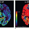
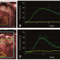
Figure 7-4. Arterial input functions (AIFs) measured in different segments of the middle cerebral artery (MCA) for data acquired using GE EPI imaging at 3T. The top row indicates the locations of the MCA segments used to measure the AIF (see arrows): (A) M1 segment, (B) M2 segment, (C) M3 segment. The corresponding AIF curves are shown in (D), with the AIF for the M1 segment labeled with crosses, the M2 segment with open circles, and the M3 segment with filled squares. Note: for comparison purposes, all AIF curves were normalized to the same area. Due to signal truncation effects, the AIF is severely underestimated in the M1 segment location. (Figure previously published in Calamante F. Arterial input function in perfusion MRI: a comprehensive review. Prog Nucl Magn Reson Spectrosc 2013;74:1-32, reprinted with permission of Elsevier, © 2013.)

While a very simple concept in theory, the measurement of the AIF is in practice a very challenging task. It can be subject to a number of major sources of error for DSC-MRI quantification, including PVE, bolus delay and dispersion, nonlinearities, truncation effect, and voxel-shift signal artifacts, among others (see also section Sources of Error and Technical Limitations below). The reader is referred to a recent review article for a detailed description of all the main sources of error in the AIF.¹⁷

In practice, a single estimate of the AIF for the whole brain (the so-called global AIF) is obtained from measuring the changes in R₂* in and around a medium-size artery, such as the M1 or M2 segment of the middle cerebral artery (MCA) at 1.5T and the M2 or M3 segments at 3T (Fig. 7.4).^c This provides a reasonable compromise between PVE, proximity to the tissue of interest, and saturation

In general, measurement of the AIF requires a reasonable level of expertise by the user and, given its central role in perfusion quantification, errors in the measured AIF can have major consequences.¹⁷ Given that the AIF represents the input to the tissue, it is often identified by a searching criterion based on a combination of features of the concentration time course. For example, an AIF is expected to have an earlier arrival, a sharper rise, earlier TTP, higher MPC, and higher peak area than the tissue voxels. Performing this search in a manual way relies on highly trained local staff, and, even in that case, it is very subjective and can be very time consuming. It is for this reason that several automatic methods have been developed to measure the global AIF (Fig. 7.5).¹⁸,¹⁹,²⁰,²¹ and ²² These software tools search through the data set to identify voxels that satisfy a criteria similar to the one used for manual AIF measurement, that is, a criteria based on a combination of temporal and shape features of the measured bolus passage, in order to choose arterial-like curves. The use of these automatic methods is highly recommended because they help to improve reproducibility, remove subjectivity, ensure site quality consistency, and allow for advanced analysis methods to be widely applied, even in centers with limited specialist expertise.

▪ From Convolution to Deconvolution

As expected, the shape of the bolus passage measured in the tissue is highly dependent on the input bolus, that is, on the AIF: the wider the input bolus, the wider the tissue concentration (for all other parameters unchanged). The tissue shape is, however, also influenced by the amount of blood delivered to the tissue (i.e., perfusion) and by other intrinsic tissue properties, which describe how the contrast agent is washed out from the capillary bed. For example, the wider the input bolus and/or the slower the washout
of contrast agent, the wider the shape of the bolus in the tissue. Similarly, the higher the blood flow rate, the larger the shape of the bolus.

Figure 7-5. Illustration of the workflow in an automatic arterial input function (AIF) searching algorithm based on cluster analysis. In (A) and (B), voxels and curves are color coded based on their area under the concentration time course. In (A), all concentration time curves are shown, and in (B), only 10% of the curves with the largest area are included. The set of curves in (B) standardized to unit area are displayed in (C) and colored according to roughness; in (D), the 25% most irregular curves have been removed. The set of curves in (D) are then partitioned into five clusters such that the intracluster variance is minimized and the intercluster variation is maximized. The partition is indicated in (E). The mean curve in the group of light blue curves had the lowest first moment and was, therefore, picked out by the algorithm and divided into five subclusters (not shown). The estimate of the AIF returned by the program was the mean curve with the lowest first moment, which is shown in (F) along with the anatomic location of the selected voxels. (Figure kindly provided by Dr. Kim Mouridsen, and reproduced from Mouridsen K, Christensen S, Gyldensted L, Ostergaard L. Automatic selection of arterial input function using cluster analysis. Magn Reson Med 2006;55(3):524-531, with permission of Wiley-Liss, Inc., © 2006.)

Therefore, the shape of the tissue concentration is dependent on three main quantities: (i) the shape of the input bolus, (ii) the delivery rate of blood, and (iii) how fast/slow the contrast leaves the tissue through the veins. From a modeling point of view, DSC-MRI quantification is based on the principles of indicator dilution theory,²³ which relates these three quantities to the tissue concentration. Based on this theory, the concentration time course in the tissue is related to the AIF by a convolution equation:

where C_AIF(t) is the AIF, R(t) is the tissue residue function, and ? is the mathematical convolution operator. The tissue residue function is an idealized mathematical concept, which describes the wash-out of the contrast agent from the tissue for the ideal case of an instantaneous bolus injection at time t = 0. In other words, for an ideal injection (i.e., an AIF corresponding to an instantaneous injection), the residue function (scaled by CBF) would correspond to the measured C(t), which describes the amount of contrast agent remaining in the tissue at time t. For this reason, the CBF-scaled residue function is also known as the “impulse response function,” that is, the function describing the response of the system to an instantaneous input bolus.

While the mathematical convolution can be a very obscure concept for nontechnical readers, it simply describes that the tissue
concentration at time t, that is, C(t), can be calculated from the superposition of contributions from an AIF considered as a consecutive series of instantaneous ideal injections (Fig. 7.6). The residue function in the convolution Eq. (3) indicates how much of each of those consecutive ideal input functions remains in the tissue at time t, whose combination leads to the measured tissue concentration at time t. The reader is referred to Calamante et al.²⁴ for a detailed review of the deconvolution process in DSC-MRI.

Figure 7-6. Schematic illustration of the role of convolution in DSC-MRI. A: Schematic AIF curve. B: Schematic tissue residue function curve. C: Discretization of the convolution expression. The top left plot in (C) shows the AIF represented as a series of consecutives discrete small inputs (as represented by the various colored bars). When each of these discrete inputs is multiplied by the corresponding residue function (i.e., the same residue function curve, but shifted to have the same delay, as shown by the curves in the bottom left plot in (C) with the colors corresponding to the colors of the discrete AIFs) and then scaled by CBF, it gives the tissue concentration time course (rightmost plot in (C)) corresponding to that discrete input. Therefore, the sum of these contributions gives the total tissue residue function, as shown in the right plot in (C). Note that for the exact convolution, the discretization is done for an infinitesimally short time interval, with an infinite number of these inputs (cf. only seven discretized inputs are shown in (C)).

Quantification of perfusion using DSC-MRI therefore requires inverting the expression in Eq. (3) to calculate CBF. From a mathematical point of view, inversion of a convolution expression is known as a “deconvolution” analysis. The concepts of convolution and deconvolution are, therefore, central to the model and analysis used in DSC-MRI, and a typical DSC-MRI experiment to quantify CBF always involves a measurement of an AIF and a deconvolution step.

Regularization

The major difficulty with inverting Eq. (3) is that deconvolution is an ill-posed problem,²⁴,²⁵ in that even a very small amount of noise in the data makes the deconvolution step extremely unreliable. Therefore, deconvolution requires, in practice, special consideration to make the solution more physically meaningful. This process is known as “regularization” of the deconvolution.

There are many ways to implement the regularization, and in all cases, this involves discarding some of the high-frequency information, which has the highest noise sensitivity. From this point of view, regularization could be thought of as type of “filtering,” but one that occurs during the deconvolution step. As with standard filtering, too little filtering leads to very unstable solutions, while too much filtering leads to oversmoothing of the solution (Fig. 7.7). The same applies to the deconvolution case, and determining the optimal amount of “filtering” (i.e., the optimal degree of regularization) is a very complex issue. In particular, the optimal level depends on many factors such as the SNR and the TR, and it even depends on tissue properties such as the CBF we are trying to quantify.²⁶,²⁷,²⁸,²⁹,³⁰,³¹,³²,³³,³⁴ and ³⁵

In general, there are two main ways in which the degree of regularization is applied in practice. Either it is fixed, based on some previously optimized values,²⁶ or it is adapted to the data based on data quality (i.e., a data-driven approach).³⁰,³¹ and ³²,³⁴,³⁶,³⁷,³⁸ and ³⁹ An example of the former case is the traditional truncated singular value decomposition (SVD) approach,²⁶ where a fixed threshold is used for every voxel in the brain and for every patient (e.g., a 20% cutoff for the SVD expansion). An example of a data-driven approach is the so-called oSVD method,³¹ a modification of the traditional SVD approach to make it delay insensitive, where a threshold for an oscillation index of the estimated residue function is used to determine the degree of regularization (i.e., the data are regularized until a certain level of smoothness is achieved based on an oscillation index). Data-driven approaches have the obvious advantage that regularization is more optimally adjusted to the available data quality (e.g., higher-quality data require less regularization than lower SNR data). However, this most often comes at the expense of larger processing times. For some applications, for example, acute stroke, the increased computation time is not a practical option (see also section DSC-MRI Analysis: Practical Implementation), which is the main reason why the faster fixed regularization approach has been more widely used.

The development of deconvolution algorithms for DSC-MRI has been a very active field of research. Most of the methods currently in
use are based on the so-called model-independent approach, where the shape of the residue function is also considered an unknown when performing the deconvolution. Model-independent methods include those based on SVD or its variants,²⁶,²⁷,³¹,⁴⁰ Fourier transform-based methods,²⁶,⁴¹ Tikhonov regularization,³² iterative algorithms,²⁸,³⁴,³⁸ Bayesian-based methods,³⁰,³⁹ among many others.⁴²,⁴³ and ⁴⁴ Each of these methods has some advantages and disadvantages regarding their accuracy, precision, processing speed, ease of implementation, sensitivity to the presence of bolus delay, etc. In fact, there is unfortunately no method currently available that is superior to all others in every single aspect, which is probably the reason why this field of research has been very active and there is no clear consensus as to what deconvolution method is preferable. In practice, the properties of the method that is given higher priority and, therefore, the actual choice of deconvolution algorithm are dependent on the specific circumstances and application. For example, if the patient population under study is likely to have considerable bolus delay (e.g., patients with severe carotid stenosis or occlusion),⁴⁵,⁴⁶ and ⁴⁷ then delay insensitivity should be among the highest priority for the criteria used to select a deconvolution method. Similarly, if data quality is very variable (e.g., in a multicenter study), then use of a data-driven regularization method should be essential.

Figure 7-7. Example of regularization using Tikhonov for simulated data. The surface plot shows the Tikhonov solutions for the tissue residue function R(t) obtained for various regularization values (with increasing regularization for increasing value of the parameter ?). The vertical axis corresponds to the Tikhonov solution R(t) and its initial value (corresponding to the blue line at time = 0) to the estimated CBF. For this particular case, the optimal solution (as determined by the corner of the L curve criterion)³² corresponds to the red curve, which is indicated by the arrows. Note that with low regularization (left side of the surface plot), there are large oscillations, and with high regularization (right side of the surface plot), the solution is oversmoothed, leading to reduced CBF estimate, as indicated by the decreasing values of the blue line with increasing regularization. (Modified from a Figure previously published in Calamante F, Gadian DG, Connelly A. Quantification of bolus-tracking MRI: Improved characterization of the tissue residue function using Tikhonov regularization. Magn Reson Med 2003;50(6):1237-1247, reprinted with permission of Wiley-Liss, Inc, © 2003.)

▪ DSC-MRI Parameters

There are a large number of hemodynamic parameters that have been calculated based on DSC-MRI data. These can be broadly divided into parameters that can only be calculated following a deconvolution analysis and those that can be calculated directly from the DSC-MRI data, often referred to as summary parameters.¹⁴ It should be emphasized that all these parameters can be calculated from the same measured DSC-MRI data, just by varying the way the data are analyzed (i.e., different postprocessing methods). This represents one of the strengths of DSC-MRI and highlights the wealth of information that can be obtained from a relatively short MRI acquisition time.

Summary Parameters

These are the DSC-MRI parameters that can be calculated without requiring a deconvolution step. They represent properties of the measured signal time course or the concentration time curve. For example, there is a number of temporal summary parameters, including TTP, bolus arrival time, full width at half maximum, and the first moment of the curve. Apart from the bolus arrival time, all these temporal parameters reflect both macrovascular and microvascular properties and, therefore, cannot be interpreted as measures of perfusion status.¹⁵,¹⁶

There are also other summary parameters related to the size effect, such as MPC and the maximum signal drop, and others related to the peak area, such as the area under the curve (AUC) and the integral-to-peak area (i.e., the area of the initial part of the concentration time curve, until the maximum concentration has been reached). In particular, the area under the peak
is related to an important physiologic parameter, the cerebral blood volume (CBV):

which represents the fraction of the tissue volume occupied by the blood and is proportional to the total amount of intravascular contrast agent in the tissue. In Eq. (4), AUC(C) represents the AUC of the tissue concentration and AUC(AIF) represents the corresponding AUC of the AIF. The normalization to the AIF is required to account for the amount of injected contrast agent. It should be noted that, for absolute quantification, the AUC ratio in Eq. (4) must be scaled by a factor describing the difference in hematocrit between arteries and capillaries and by the density of brain tissue.¹⁴

Deconvolution-Related Parameters

The main parameter in this case is CBF, which can be calculated, in principle, from the initial value of the impulse response function, CBF × R(t). This follows from the fact that, by definition, R(t = 0) = 1, that is, all the contrast agent is present in the tissue at t = 0 following the injection of an ideal input bolus a t = 0. In practice, however, the shape of the impulse residue function can be subject to a number of artifacts,⁴⁸ including bolus dispersion and deconvolution errors (see section Sources of Error and Technical Limitations for more details). In particular, bolus dispersion makes the initial value of the impulse response function equal to zero.⁴⁹ It is for this reason that, in practice, CBF is most often estimated from the maximum of the impulse function rather than from its initial value.²⁶,⁴⁹

There are two further deconvolution-related parameters that are often calculated in DSC-MRI studies and that reflect temporal features: the mean transit time (MTT) and T_max. MTT corresponds to the average time it takes the blood (and therefore the contrast agent) to travel through the tissue capillary network following the injection of an ideal bolus. MTT can be calculated based on the central volume theorem²³ as the ratio of blood volume to blood flow:

In turn, T_max represent the time to maximum of the impulse response function⁵⁰ and corresponds, in theory, to the bolus delay.⁵¹ However, in practice, because a number of artifacts can distort the shape of the calculated impulse response function (see section Sources of Error and Technical Limitations for more details), T_max can be also influenced by bolus dispersion and, to a smaller extent, by MTT.⁵¹ It should therefore be considered primarily a measure of macrovascular status. This parameter has increasingly being used in stroke imaging, and it has been one of the parameters of choice for several major stroke clinical trials.⁵²,⁵³,⁵⁴ and ⁵⁵

▪ Absolute Quantification

DSC-MRI has been often criticized as a technique that can only measure CBF in relative units.⁵⁶,⁵⁷ While this view was correct earlier on, technical developments in this field have made considerable progress in recent years, and DSC-MRI has now grown to be a perfusion imaging technique that can provide robust measurements in absolute units (e.g., in mL/100 g/min).

To obtain perfusion in absolute units, it is most often necessary to scale the results from the deconvolution analysis (which can be considered to be in arbitrary units, or “DSC units”) to CBF measurements in absolute units.^d It is essential, however, that this scaling is carried out using a patient-specific scaling factor. This scaling factor is aimed at compensating for scaling errors due to several factors, such as nonlinearities, and PVE (see section Sources of Error and Technical Limitations for more details), which cannot be assumed uniform across patients. Several methods that provide a patient-specific scaling have now been proposed.⁵⁸,⁵⁹,⁶⁰,⁶¹,⁶² and ⁶³ The scaling is usually calculated from data obtained using an extra MR data set. For example, the first method proposed, the “bookend technique,”⁵⁸,⁵⁹ calculates the scaling factor from a T₁-based CBV measurement obtained from two extra T₁ maps acquired just before and after DSCMRI (i.e., pre- and postcontrast agent T₁ measurements). This CBV map (which is in absolute units because it is based on T₁ data)⁶⁴ can be compared with the relative CBV map from DSCMRI, to obtain a “bookend” scaling factor that can be applied to the CBF map.

Other alternative methods to obtain the patient-specific scaling relies, for example, on an extra regional CBF measurement from ASL data, with a method known as “combined ASL and DSC CBF” (CAD-CBF),⁶⁰ or on the total cerebral flow calculated from a complementary phase-contrast MR angiography (MRA) measurement.⁶¹ In both cases, the extra measurement is used to calculate the required scaling for the CBF map from DSC-MRI on a patient-bypatient basis. Other further methods are based on scaling factors based on ratio measurements between the veins and the arteries, such as by using the venous output function (a function similar to the AIF but that characterizes the output of the bolus from the tissue, rather than the input)⁶² or by using the pseudo-steady-state contrast concentration after the first pass (i.e., the measured concentration during the tail of the peak).⁶³

These subject-specific scaling methods are in contrast to early attempts to convert to absolute units, using methods that relied in a uniform scaling factor for all patients.⁴¹,⁴²,⁶⁵,⁶⁶ The most common of these earlier methods was based on scaling the maps by fixing to 22 mL/100 g/min the CBF value of a reference region in contralateral white matter.⁶⁵ Any of these approaches that rely on a uniform scaling factor are strongly discouraged for clinical applications where absolute units are required.

Only gold members can continue reading. Log In or Register to continue