Echo Planar Imaging
Introduction
In the last three chapters, we discussed some of the fast scanning techniques, namely, the fast spin echo (FSE) and gradient-recalled echo (GRE) techniques along with their “fast” variants. In this chapter, we will discuss the echo planar imaging (EPI) technique, which is the fastest MRI technique available.
Basic Idea in EPI
Unlike other fast scanning techniques that can be achieved via software updates, single-shot EPI requires hardware modifications. More specifically, high performance gradients (discussed in Chapter 30) are needed to allow rapid on-andoff switching of the gradients. The basic idea is to fill k-space in one shot (single-shot EPI) with readout gradient during one T2* decay (if longer, T2 blurring will occur) or in multiple shots (multishot EPI) by using multiple excitations. As we shall see shortly, single-shot EPI allows oscillating frequency-encoding gradient pulses and complete k-space filling after a single RF pulse. Generally, gradient strengths of over 20 mT/m and gradient rise times of less than 300 µsec are required. Furthermore, extremely fast computers are needed to allow fast digital manipulations and signal processing.
Types of EPI
Two main types exist: single-shot EPI and multishot EPI. Earlier single-shot EPI techniques used a constant phase-encode gradient. Newer techniques use a “blipped” phase-encode gradient, referred to as “blipped EPI.”1
Single-Shot EPI. In single-shot EPI, all the lines in k-space are filled by multiple gradient reversals, producing multiple gradient echoes in a single acquisition after a single radio frequency (RF) pulse, that is, in a single measurement or “shot.”
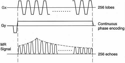
To achieve this, the readout gradient must be reversed rapidly from maximum positive to maximum negative Ny/2 times (e.g., 256/2 = 128 times) during a single T2* decay (e.g., 100 msec). Each lobe of the readout gradient above or below the baseline corresponds to a separate ky line in k-space. Therefore, the number of phase-encode steps Ny is equal to the sum of the positive and negative lobes of the readout gradient. The area under the Gx lobe determines the field of view (FOV)—the larger the area, the smaller the FOV. Apparently, single-shot EPI places tremendous demands on the gradients with respect to maximum strength Gmax and minimum rise time tRmin (i.e., the maximum slew rate Gmax/tR) as well as on the analogto- digital converter (ADC). In general, ADCs with maximum bandwidths (BWs) on the order of MHz are required rather than the kHz maximum BWs used for conventional spin echo (CSE).
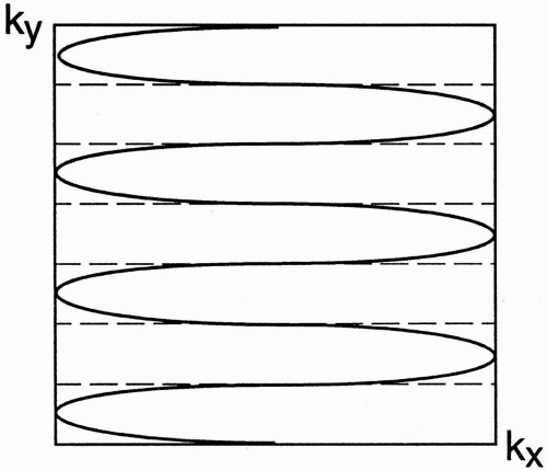
In earlier EPI methods, the phase-encode gradient was kept on continuously (Fig. 22-1)
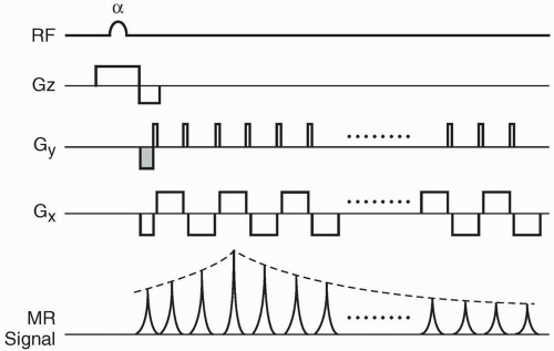
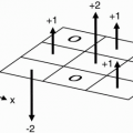
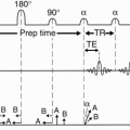
during the acquisition, resulting in the zigzag coverage of k-space (Fig. 22-2). This led to some artifacts during Fourier transformation compared with conventional k-space trajectories. To rectify this problem, the phase-encode gradient was subsequently applied briefly during the time when the readout gradient was zero, that is, when the k-space position was at either end of the kx axis (Fig. 22-3). This method was referred to as blipped phase encoding, as its duration was minimal (200 µsec). Therefore, the same phase-encode gradient is applied briefly Ny number of times (e.g., 256 times). The technique was called blipped EPI, and the k-space trajectory (Fig. 22-4) was much easier on the Fourier transformation.
during the acquisition, resulting in the zigzag coverage of k-space (Fig. 22-2). This led to some artifacts during Fourier transformation compared with conventional k-space trajectories. To rectify this problem, the phase-encode gradient was subsequently applied briefly during the time when the readout gradient was zero, that is, when the k-space position was at either end of the kx axis (Fig. 22-3). This method was referred to as blipped phase encoding, as its duration was minimal (200 µsec). Therefore, the same phase-encode gradient is applied briefly Ny number of times (e.g., 256 times). The technique was called blipped EPI, and the k-space trajectory (Fig. 22-4) was much easier on the Fourier transformation.
 |
As discussed previously, one of the problems with single-shot EPI is that any phase error tends to propagate through the entire kspace. (This is not a problem in CSE because of the presence of rewinder gradients, which reset the phase at the end of each cycle.) The phase errors we are talking about here are not the ones caused by motion (motion artifact is not a problem in the ultrafast EPI) but the errors arising from the variation in the resonating frequencies of protons (e.g., fat and water protons), which lead to mismapping along the phase-encode axis. Consequently, one of the technical problems of single-shot EPI is magnetic susceptibility artifacts, particularly at air/tissue interfaces around the paranasal sinuses. Also, because of this phase error propagation along the phase-encode axis, chemical shift artifact in EPI is along the phase-encode axis rather than the frequency-encode axis, as in the case of CSE.
 |
 |
Multishot EPI. In multishot EPI, the readout is divided into multiple “shots” or segments (Ns), so that Ny = Ns × ETL where ETL (echo train length) is the number of lines in each segment. Because k-space is segmented into multiple acquisitions, this technique is also called segmental EPI.
This technique places less stress on the gradients compared with single-shot EPI.
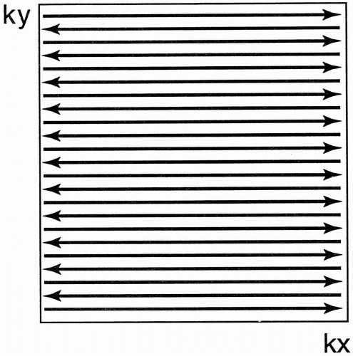
Figure 22-4. The k-space trajectory for blipped EPI in an odd-even manner, which is much easier on the Fourier transformation.
Phase errors have less time to build up compared with single-shot EPI, thus reducing diamagnetic susceptibility artifacts.
Because of this fact, multishot EPI is more susceptible to motion artifacts.
Pulse Sequence Diagram in EPI
Figure 22-1 illustrates an example of the original EPI pulse sequence diagram (PSD). The major difference between this sequence and a conventional sequence is the application of a series of sinusoidal-shaped pulse sequences along the readout axis. This series requires rapid on-andoff switching of the gradients to achieve a train of positive and negative gradient pulses. It can be accomplished only with advanced hardware that can support such high performance gradients. The other difference is the application of a constant phase-encoding gradient (remember that k-space is filled in one TR period). (The term TR may not be suitable here because each slice is obtained after a single RF pulse. However, TR could be defined as the time between successive slice-select RF pulses.) The above scheme allows acquisition of raw data for each slice after a single RF pulse (unlike routine SE, in which one RF pulse is needed for each phase-encoding step).
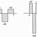
Figure 22-3 provides a PSD for blipped EPI in which the phase-encode gradient is applied briefly Ny number of times when the readout gradient is zero.
k-Space Trajectory in EPI
Unlike CSE


Related posts:
Stay updated, free articles. Join our Telegram channel
Full access? Get Clinical Tree
