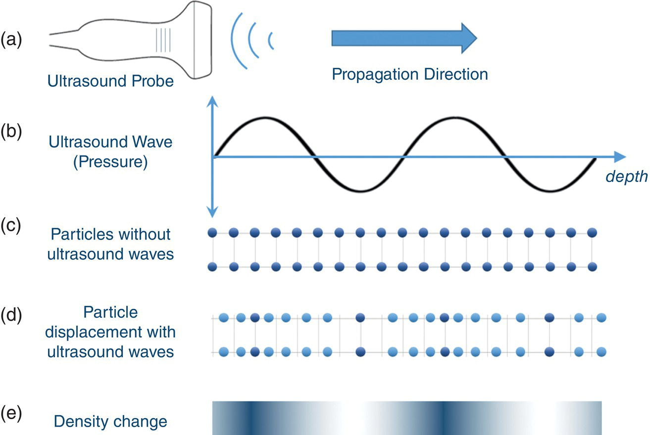
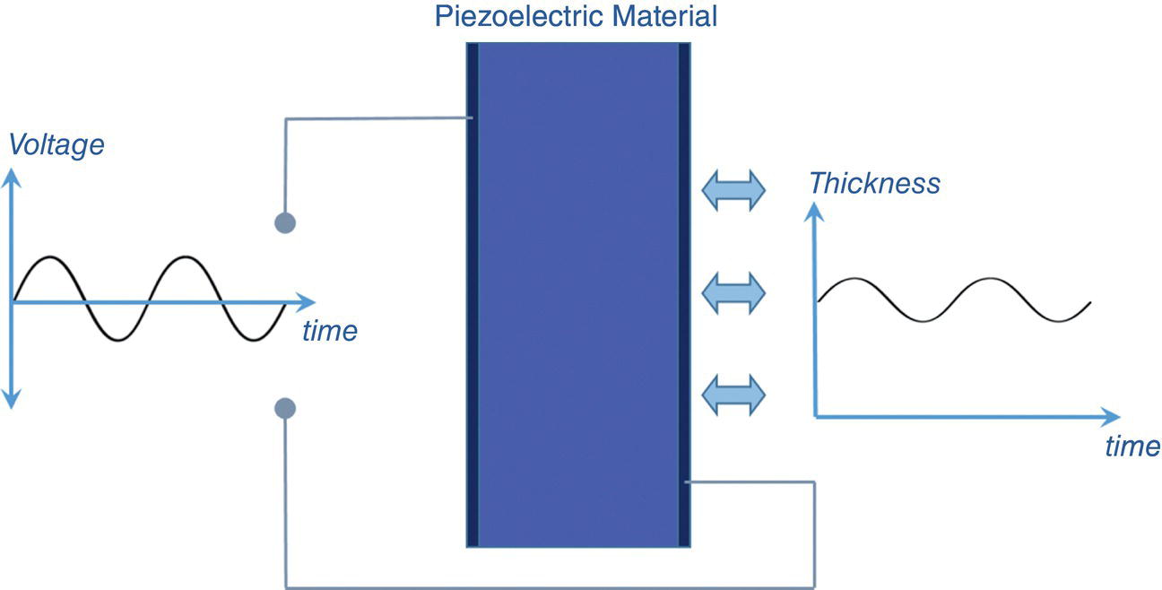
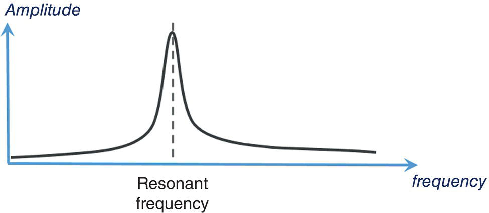
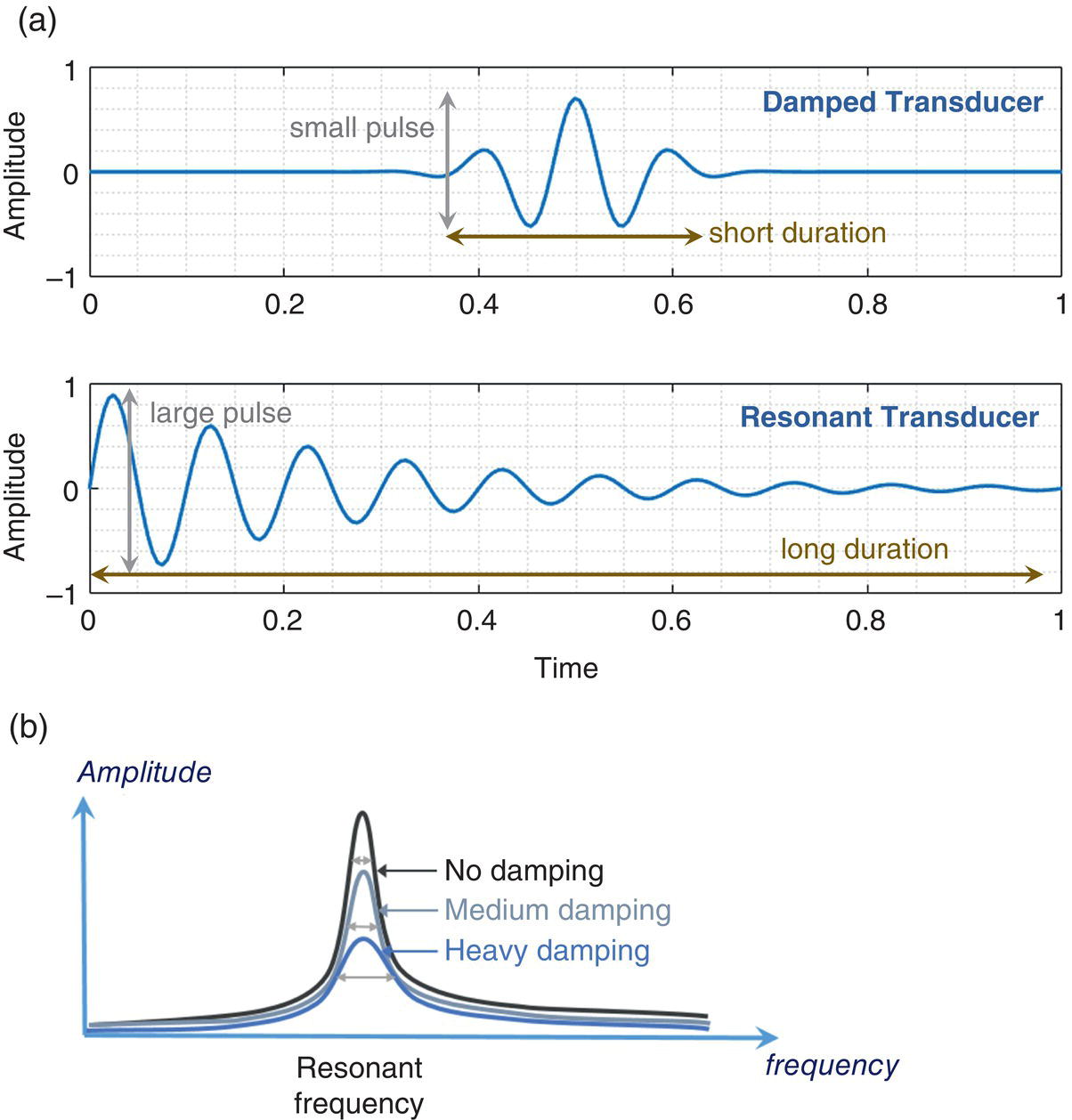
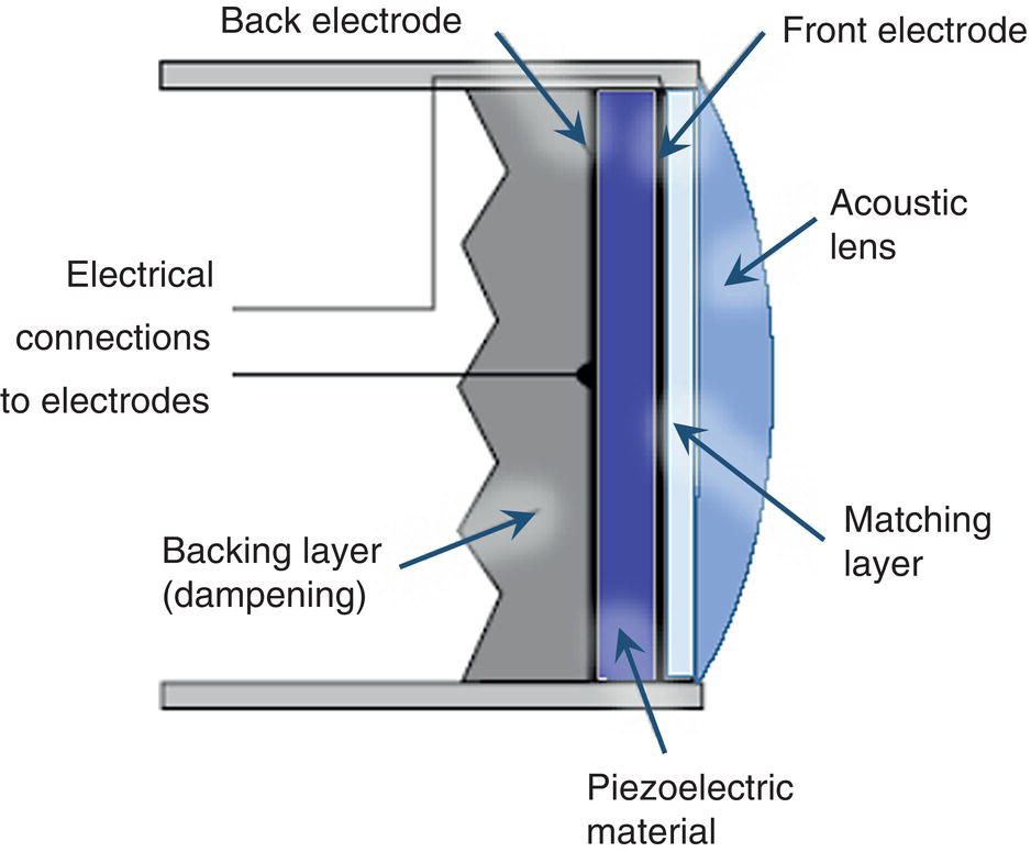
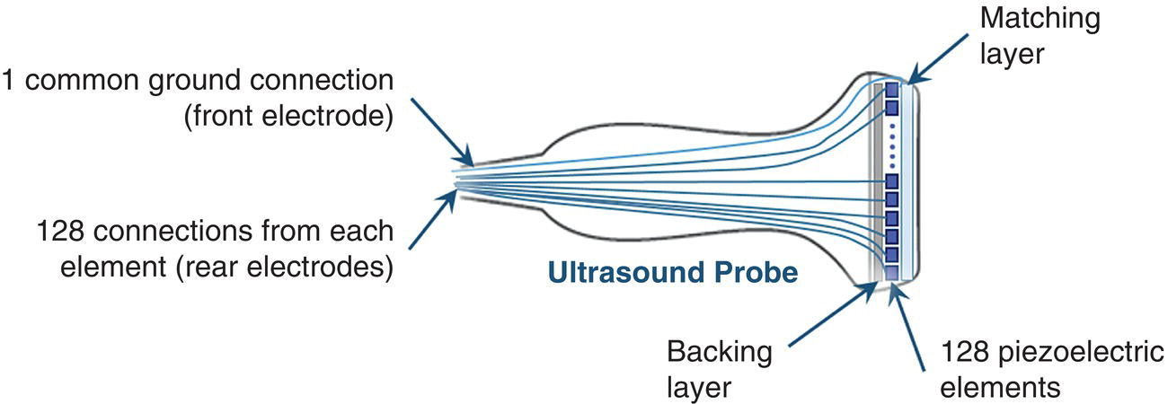
Sevan Harput1, Xiaowei Zhou2, and Meng‐Xing Tang3 1 Division of Electrical and Electronic Engineering, London South Bank University, London, UK 2 State Key Laboratory of Ultrasound Engineering in Medicine, College of Biomedical Engineering, Chongqing Medical University, Chongqing, China 3 Department of Bioengineering, Imperial College London, UK Ultrasound refers to an acoustic wave whose frequency is greater than the upper limit of human hearing, which is usually considered to be 20 kHz. Medical ultrasound operates at a much higher frequency range (generally 1–15 MHz) and it is inaudible. Medical ultrasound images are produced based on the interaction between the ultrasound waves with the human body. For this reason, producing and interpreting an ultrasound image require an understanding of the ultrasound waves, their transmission and reception by sensors, and the mechanisms by which they interact with biological tissues. Unlike electromagnetic waves used in optical imaging, X‐ray, and computed tomography (CT), ultrasound waves are mechanical waves that require a physical medium to propagate through. For example, ultrasound waves can travel in water or human tissue, but not in a vacuum. Ultrasound waves transport mechanical energy through the local vibration of particles. In other terms, an ultrasound wave propagates by the backwards and forwards movement of the particles in the medium. It is important to note that while the wave travels, the particles themselves are merely displaced locally, with no net transport of the particles themselves. For example, if a lighted candle is placed in front of a loudspeaker, the flame may flicker due to local vibrations, but the flame would not be extinguished since there is no net flow of air, even though the sound can travel far away from the speaker [1]. While propagating in a medium, both the physical characteristics of the ultrasound wave and the medium are important for understanding the wave behaviour. Therefore, this section will first introduce the relevant physical processes and parameters that affect ultrasound wave propagation. There are many types of acoustic waves, such as longitudinal, shear, torsional, and surface waves. The mechanical energy contained in one form of an acoustic wave can be converted to another, so most of the time these waves do not exist in isolation. However, for the sake of simplicity we will only describe the longitudinal or compressional waves, which are most commonly used in B‐mode and Doppler imaging. The propagation of longitudinal ultrasound waves is illustrated in Figure 1.1 using discrete particles. As we know, human tissue is not made up of discrete particles, but rather a continuous medium with a more complicated structure. This is merely a simplified physical model to explain wave propagation. During the wave propagation, particles are displaced due to the acoustic pressure in parallel to the direction of motion of the longitudinal wave, as illustrated in Figure 1.1a–c. When the pressure of the medium is increased by the wave, which is called the compression phase, particles in adjacent regions move towards each other. During the reduced pressure phase (rarefaction), particles move apart from each other. During these two phases, the change in the concentration of particles changes the local density, shown in Figure 1.1d as the higher‐density regions with darker colours. This change in local density can be related to the change in acoustic pressure, which is also proportional to the velocity of the particles, Figure 1.1e. Particle velocity should not be confused with the speed of sound. The ultrasound wave travels, while the particles oscillate around their original position. The particle velocity is relatively small in comparison to the speed of sound in the medium. Figure 1.1 (a–e) Longitudinal wave propagation using a simplified physical model depicted graphically. A detailed explanation is in the text above. A propagating ultrasound wave can be characterised by its speed, frequency, and wavelength. Similar to other types of waves, the speed of propagation of an ultrasound wave is determined by the medium it is travelling in. Propagation speed is usually referred to as the speed of sound, denoted by ‘c’, and it is a function of the density, ‘ρ’, and stiffness, ‘k’, of the medium, as shown in Equation 1.1: Tissue with low density and high stiffness has a high speed of sound, whereas high density and low stiffness lead to low speed of sound. See Table 1.1 for speed of sound values in different tissue types and materials [2, 3]. In addition to speed of sound, the frequency, ‘f’, and the wavelength, ‘λ’, of the ultrasound wave are crucial parameters for medical ultrasound imaging. The frequency of a wave is the reciprocal of the time duration of a single oscillation cycle of the wave and carries a unit of Hz. The wavelength is the length of a single cycle of the wave and is linked to frequency and speed of sound, as in Equation 1.2: In short, frequency has the timing information about the wave for a given space, and wavelength has the spatial (relating to physical space) information about the wave at a given time. Ultrasound image resolution is related to frequency/wavelength and is usually better at higher frequencies and shorter wavelengths. At a given ultrasound imaging frequency, the wavelength changes proportionally with the speed of sound. For medical ultrasound imaging, the speed of sound is usually assumed to be constant for the tissue and in order to change the image resolution, one needs to change the imaging frequency. For example, for an average speed of sound in soft tissues of 1540 m/s, the wavelength is 0.77 mm at 2 MHz and 0.154 mm at 10 MHz. Table 1.1 Ultrasound properties of common materials and tissue. Acoustic impedance is the effective resistance of a medium to the applied acoustic pressure. For example, the particle velocity in soft tissue will be higher than the particle velocity in bone for the same applied pressure due to the difference in their acoustic impedance (see Table 1.1). The acoustic impedance, ‘Z’, of a material is determined by its density and stiffness values, as shown in Equation 1.3: When an ultrasound wave travelling through a medium reaches an interface of another medium with a different acoustic impedance, some portion of the ultrasound wave is reflected, as shown in Figures 1.2 and 1.3. The amplitudes of the transmitted and reflected ultrasound waves depend on the difference between the acoustic impedances of both media, see Figure 1.3. This can be formulated as the reflection coefficient, shown in Equation 1.4: The interfaces with higher reflection coefficients appear brighter on an ultrasound B‐mode image, since a large portion of the ultrasound wave is reflected back. Reflection coefficients at some common interfaces are shown in Table 1.2. It should be remembered that the underlying model for the equation of the reflection coefficient is based on specular reflection, which means a reflection from a perfectly flat surface or an interface. In reality, the reflection of ultrasound waves can be considered either specular or diffuse (https://radiologykey.com/physics‐of‐ultrasound‐2). When the ultrasound waves encounter a large smooth surface such as bone, the reflected echoes have relatively uniform direction. This is a type of specular reflection, as shown on the left of Figure 1.2. When the ultrasound waves reflect from a soft tissue interface, such as fat–liver, the reflected echoes can propagate towards different directions. This is a type of diffuse reflection, as shown on the right of Figure 1.2. Refraction is the bending of a wave when it enters a medium with a different speed. It is commonly observed with all types of waves. For example, when looked from above, a spoon appears to be bent in a glass full of water. The reason for this is that the light emerging from the water is refracted away from the normal, causing the apparent position of the spoon to be displaced from its real position, due to the difference in the speed of light in water and in air. Figure 1.2 Specular (left) and diffuse (right) reflection. Refraction of ultrasound waves occurs at boundaries between different types of tissue (different speeds of sound), as shown in Figure 1.3. In ultrasound imaging, this can cause displacement of the target from its true relative position. If the speed of sound is the same in both media, then the transmitted ultrasound wave carries on in the same direction as the incident wave. Human tissue has inhomogeneities. When these inhomogeneities are much smaller than the wavelength, then the ultrasound wave is scattered in many directions, as shown in Figure 1.3. Most of the ultrasound wave travels forward and a certain portion of the wave’s energy is redirected in a direction other than the principal direction of propagation. Scattering reduces the amplitude of the initial propagating ultrasound wave, but the lost energy due to scattering is not converted to heat. Table 1.2 Reflection coefficients at some common interfaces. Figure 1.3 (a) Reflected, refracted, and (b) scattered waves. Scattering plays an important role in blood velocity estimation. Blood cells (e.g. erythrocytes are 6–8 μm) are usually much smaller than ultrasound imaging wavelengths (>100 μm). Therefore, blood does not reflect but scatter the ultrasound waves. Ultrasound waves are pressure waves. They change the local density by compression and rarefaction, where not all adjacent particles move together. When particles are moving towards each other they experience friction. In medical imaging, this friction is caused by the viscoelastic behaviour of human soft tissue, which is effectively the resistance against the motion. When the local compression generated by the ultrasound waves are resisted by the friction of the soft tissue, heat is generated. In other words, there will be tiny differences in temperature between regions of compression and rarefaction. Tissue will conduct heat from the higher‐temperature region to the lower. This overall process will result in a bulk rise in temperature of the tissue due to viscous losses. Consequently, the energy of the travelling ultrasound waves will be lost after propagation. Attenuation means a reduction in the amplitude of ultrasound waves. In ultrasound imaging, attenuation of the transmitted waves is usually as a result of absorption, but other physical processes also attenuate the waves, such as reflection, refraction, scattering, and diffraction. The amount of attenuation is usually expressed in terms of the attenuation coefficient, as shown in Table 1.1. The most important practical implication of attenuation is that it is hard to achieve good resolution in deep tissue. The image spatial resolution is better at higher ultrasound frequencies. However, the attenuation in tissue is also higher at higher frequencies. Over a given distance, higher‐frequency sound waves have more attenuation than lower‐frequency waves. This results in a natural trade‐off between image resolution (frequency) and imaging depth (penetration). The functionalities to increase the signal amplification with depth in all ultrasound systems, known as time gain compensation (TGC), can, to a limited extent, recover weak signals in deep tissues. A transducer is a device that converts one type of energy into another. An ultrasound transducer generates ultrasound waves by converting electrical energy into mechanical energy. Conversely, an ultrasound transducer can convert mechanical energy into electrical energy. This duality is particularly useful for imaging applications, where the same ultrasound transducer can generate ultrasound waves and also sense the reflected echoes from the human body. Inside all ultrasound imaging probes there are transducer elements that convert electrical signals into ultrasound and, conversely, ultrasonic waves into electrical signals. There are several different methods to fabricate an ultrasound transducer. In this section, we will only explain the piezoelectric materials, which are used in most ultrasound probes. In precise terms, piezoelectric materials work with the principle of piezoelectric effect, which is the induction of an electric charge in response to an applied mechanical strain. The piezoelectric effect explains how ultrasound sensors can detect pressure changes. This effect may be reversed, and the piezoelectric material can be used to generate pressure waves by applying an electric field. Figure 1.4 Changes in voltage across both sides of the piezoelectric material causes changes in the thickness. Ultrasound waves can be generated by applying an alternating current (AC) with a frequency closer to the working frequency of the transducer. The AC voltage produces expansions and contractions of the piezoelectric material, which eventually create the compression and rarefaction phases of the ultrasound waves, as shown in Figure 1.4. Usually the displacement on the surface of the piezoelectric material is proportional to the applied voltage. When pressure is applied to the piezoelectric material, it produces voltage proportional to the pressure. The frequency at which the transducer is most efficient is the resonance frequency. The transducer is also the most sensitive as a receiver at its resonance. If the applied voltage is at the resonance frequency of the transducer, it generates ultrasound waves with the highest amplitude, as shown in Figure 1.5. The thickness and shape of the piezoelectric material determine the resonance frequency of the ultrasound transducer. The same piezoelectric material can be cut and shaped in different sizes to produce transducers working at different frequencies. Bandwidth is the range of frequencies at which the transducer can operate without significant loss. Piezoelectric materials are resonant systems that work well only at the resonance frequency, but this is not ideal for imaging applications. Imaging applications require a transducer that can work at a range of frequencies. For this reason, manufacturers apply damping to reduce the resonance behaviour. Figure 1.6 shows the response of a resonant and a highly damped transducer. The undamped transducer has unwanted ringing even after the electrical signal stops. This long‐duration response of the transducer is not ideal for imaging. A good imaging pulse has a short duration in time, so it can be used to determine objects close to each other. A short pulse contains a range of frequencies and is better accommodated by a transducer with wide bandwidth, such as the damped transducer shown in Figure 1.6. Figure 1.5 Resonance behaviour of piezoelectric ultrasound transducers. Single‐element ultrasound transducers are fabricated by using one plate of piezoelectric material, as illustrated in Figure 1.7. A thin plate of piezoelectric material (shown in dark blue) is coated on both sides with a conductive layer, forming electrodes. Both electrodes are bonded to electrical leads that are connected to an external system to transmit or receive ultrasound waves. The front electrode is usually connected to the metallic case of the transducer and the electrical ground for safety. The back electrode is the electrically active lead. In order to transmit an ultrasound wave, an oscillating voltage is applied to the electrodes. A matching layer is specifically designed for a target application, such as imaging the human body, and it increases the coupling efficiency of the transducer to the body. An acoustic lens may be placed in front of the matching layer to create a weak focal zone. This is particularly useful for small (small in comparison to the operating wavelength) transducers that diverge ultrasound waves outside the imaging region. The backing layer is specifically designed to absorb unwanted internal reverberations. It effectively dampens the resonance behaviour of the piezoelectric material and increases its bandwidth. Figure 1.6 Response of a highly resonant transducer and damped transducer to a short electrical pulse. (a) Transducer response measured as a function of time. (b) The corresponding frequency response. Figure 1.7 An ultrasound transducer’s internal architecture. A single‐element transducer can act as a transmitter and also as a receiver. This makes it possible to measure the elapsed time between the transmission of an ultrasound pulse and the reception of its echo from a reflecting or scattering target. If the speed of sound in the medium is known, then the distance to the source of the echo can be calculated. After a single measurement, the depth and the amplitude of the echo, which are related to the ultrasonic properties of the target, can be calculated. This measurement method is usually called a pulse–echo method or an A‐scan. It is possible to generate an image by moving the transducer element and performing several A‐scan measurements. However, this is not practical for imaging, since it requires a mechanical motion and knowledge of the exact transducer location in order to precisely combine the A‐scan measurements. The mechanical scanning method is slower than the electronic scanning method, which will be explained in the next section. Most clinical ultrasound imaging probes consist of an array of transducer elements. Arrays provide flexibility as the transmitted ultrasound beam can be changed on the fly, which is not possible with solid apertures or single‐element transducers. The array transducers usually have hundreds of elements with a single front electrode connecting all elements together to the electrical ground. This is important for safety and also reduces fabrication complexity. Each element has individual electrodes at the rear, and these are connected to the imaging system with a separate cable, as shown in Figure 1.8. The ultrasound system can control each element individually during the transmit and receive cycles. By controlling the timing of transmission in each element, the ultrasound beam can be focused or steered electronically at different depths and directions in so‐called transmit beamforming. Figure 1.8 Schematic of an array transducer. The most common ultrasound imaging method is line‐by‐line image formation. In this method, the ultrasound energy is focused into a long and narrow region, as illustrated by the arrows in Figure 1.9 for different type of imaging probes. The received echoes from each transmission form a single line in the ultrasound image. After completing a transmit–receive sequence, the scan line is moved to the next position. The repositioning of the scan line is achieved electronically by controlling the timing of transducer elements. Electronically scanned arrays do not have any moving parts compared to mechanically scanned solid apertures, which are slow and require maintenance. It should be noted that the ‘image line’ is in reality a 3D volume, as shown in Figure 1.9d, narrower at the focal plane and wider elsewhere. Figure 1.9 The line‐by‐line scanning approach is illustrated for different types of ultrasound probes used for liver scans. (a) Linear array. (b) Curvilinear array. (c) Phased array. (d) An imaging line. The transmitted ultrasound waves propagate through tissue and are reflected and scattered from tissue boundaries and small inhomogeneities wherever there is an acoustic impedance mismatch. A portion of these reflected and scattered ultrasound waves travels back to the transducer and is then converted to electrical signals by the transducer elements. Each element on the transducer provides a distinct electrical signal where the timing of each signal accommodates the distance information. Signals from each element are normally called channel signal. All channel signals are processed to reconstruct the images in different imaging modes with three main steps, pre‐processing to amplify signals and remove noises, receive beamforming to reconstruct the image, and post‐processing to enhance the image quality. Pre‐processing is to enhance the received signals and remove noises for each channel signal before the receive beamforming. The first step is to amplify the received channel signals, as their amplitudes are generally too small to be processed directly by a beamformer. Besides the signal pre‐amplifiers, to which users do not have access, there are two types of amplifiers that can be controlled by users: an overall amplifier and a TGC (Figure 1.10). The overall amplifier enhances the received signals as a whole, regardless of where these signals are originating from, while the TGC amplifies the signals based on the arrival time to have later‐arriving signals from deeper regions being amplified more as they are more attenuated. Although these user‐controlled amplifiers are to enhance the received signals, they also amplify the noise. To ensure a sufficient signal‐to‐noise ratio (SNR), a certain level of transmission power is required. Figure 1.10 The typical time gain compensation (TGC) slide controls for different gains at different depths. Band pass and other filters may also be used after the amplifications to remove some electrical noise in the signals. Signals received at each channel are analogue signals, which vary continuously. The beamforming and all post‐processing in modern scanners are done in digital form. Therefore, analogue‐to‐digital conversion (ADC) is always required for digital processing. In receive beamforming, the echoes received from all transducer elements are realigned in time through pre‐determined time delays, so that only the echoes originating from the same spatial locations (pixels) are summed. In clinical ultrasound scanners, the images in all modes are typically formed with line‐by‐line transmitting and receiving, so signals from each transducer element are realigned to focus at specified depth(s) for each scanning line after the ADC. The realignment is done by compensating for the arriving delay time, which is determined by the path length between the specified depth and the individual elements, as shown in Figure 1.11. Then the realigned signals corresponding to a certain spatial location (pixel) are summed. This beamforming method is called delay‐and‐sum (DAS). In order for every pixel, or depth along the scan line, to be in focus in the reconstructed image, the delays to arrival time in DAS need to be adjusted dynamically to achieve continuous advancement of the focusing depth and have what it is called ‘dynamic focusing in reception’. Figure 1.11 The delay‐and‐sum receive beamforming method for obtaining the in‐phase summation of signals from individual active elements at a specific focusing depth. ‘Dynamic focusing’ means the delays need to be calculated for multiple depths. Most ultrasound imaging modes, including B‐mode ultrasound, Doppler ultrasound, and elastography, need to have the pre‐processing and line‐by‐line receive beamforming procedure before the image display. The differences among those imaging modes start from post‐processing after line‐by‐line beamforming, which will be explained in the following sections. B‐mode ultrasound in this chapter (B stands for brightness) refers to virtualising the tissue structures based on the brightness of received signals. According to the frequency components of the received signals selected for B‐mode imaging, there is fundamental frequency imaging or harmonic imaging. When an acoustic wave propagates in the human body, in addition to the attenuation of its amplitude, its initial shape and frequency compositions can also be gradually altered by the tissue as it propagates, a phenomenon called non‐linear propagation. This is due to the fact that the local tissue density does not respond entirely proportionally to the local ultrasound compression or rarefaction pressure, especially at high acoustic pressures. Consequently, the propagating wave, as well as the received signals, not only has the same frequency components as the transmitted pulse (called fundamental frequency), but also harmonic frequencies, which are multiples of the transmitted frequencies. This distortion tends to occur when the transmitted pulse has high pressure or when there are ultrasound contrast media along the propagation path. The different frequency components of the received signals have different characteristics, and the choice of which component to use forms the basis of the two imaging approaches, fundamental frequency imaging and harmonic imaging. Image reconstruction in both categories is to be explained in this section. This imaging approach assumes that the higher harmonic frequencies in the received signals can be discarded and only considers the fundamental frequency components. After the DAS beamforming, the summed signal is still in the radio frequency (RF) domain, oscillating at the transmitted frequency when non‐linear propagation is ignored. This RF signal can be described as a modulated sinusoidal signal, which has the amplitude and phase information. In B‐mode imaging, it is the amplitude information that determines the brightness of the image; the phase information is normally discarded. A procedure called amplitude demodulation is applied to extract this envelope information by removing the oscillating carrier frequency, as shown in Figure 1.12. Envelopes from each scanning line will be used to form a two‐dimensional B‐mode image. In harmonic imaging, signals at the transmitted fundamental frequency are removed from the beamformed RF signal, and only the harmonic components are selected for extracting the envelope information and forming B‐mode images. This is typically done by filtering out the fundamental components with a bandpass filter. One of the advantages of using harmonic components is that the beam width in the lateral direction is narrower than that of the fundamental components (Figure 1.13), which will give better lateral resolution, as explained in the next section. After removing the fundamental frequency components, amplitude demodulation is also needed to extract envelopes from harmonic components in each scanning line to form the 2D image. Figure 1.12 A pulsed ultrasound beam to image two point sources along one scanning line shown on the left. (a) The beamformed radio frequency signal. (b) Amplitude modulation applied to get the envelope of the two point sources. (c) The extracted envelope on this scanning line for the image display. Figure 1.13 Computed harmonic beam profiles in the focal plane of a 2.25 MHz transducer, where lateral resolution is much improved with harmonic imaging. Source: Reproduced by permission from Duck, F.A., Baker, A.C., Starritt, H.C. (eds) (1998) Ultrasound in Medicine, Boca Raton, FL: CRC Press. When evaluating the performance of an imaging system, the user should consider three different resolutions: temporal resolution, spatial resolution, and contrast resolution. The temporal resolution is to measure how many image frames can be reconstructed per second (fps). High temporal resolution is required to capture the fast‐moving objects in the tissue, such as the moving heart and blood flow. Spatial resolution is to evaluate the ability of an imaging system to distinguish the two closest points in a 3D object space. It includes the spatial resolution in the axial direction, lateral direction, and elevational direction in the ultrasound imaging coordinates (Figure 1.14). Spatial resolution in the axial direction is determined by the length of the transmitted pulse (Figure 1.12), which in turn is determined by the central frequency of the transmission and the bandwidth of the system. In the lateral direction, the resolution is related to the lateral beam width (Figure 1.12) and depends on the size of the transducer aperture and the imaging depth; it is typically between one and two wavelengths of the transmitted waves. In the elevational direction, the resolution is determined by the thickness of the scan plane, also called slice thickness, which varies with depth. Most transducers have a fixed focusing depth in the elevational direction, achieved by a cylindrical acoustic lens attached to the transducer face. Even with the lens focusing, the slice thickness is generally larger than the beam width in the lateral direction. Figure 1.14 The conventional coordinate system in an ultrasound imaging system. Contrast resolution defines the ability to differentiate an area of tissue from its surroundings. This ability is important in ultrasound diagnosis, since it can help identify different organs and monitor pathological change. Compared to magnetic resonance imaging (MRI), ultrasound imaging has relatively less contrast resolution due to the similar echogenicity of different soft tissues in the body. Before displaying the image on the screen, it is necessary to compress the signals into a certain dynamic range. This is because the reflected intensity from different tissues spreads over a large range. If all these intensities were displayed on the screen in a linear scale, the weak echoes scattered from most soft tissues would be dark in the image, and only the echoes from large surfaces/interfaces would stand out. To address this issue, the large‐range intensity values of echoes are compressed to simultaneously display strong echoes from, for instance, organ interfaces and weak signals from within soft tissues. This compression process is normally a non‐linear procedure such as logarithm compression, which amplifies the weak echoes more than it does the large echoes. In commercial ultrasound scanners, the non‐linear compression curve can be adjusted to have a different dynamic range for the final image display. After compression, the image can be displayed on the screen for diagnosis. From ultrasound transmission to final display the whole process can be in real time. Modern commercial systems may also use some advanced filters to reduce the speckle effect in the image or further smooth the image for an improved visual display. Medical Doppler ultrasound uses ultrasonic waves for measuring blood flow in the cardiovascular system as well as tissue motion. It has been widely used in clinical practice; its high temporal resolution and real‐time imaging make it a unique modality for blood flow measurements. Over the past 50 years, most Doppler systems may be categorised as the continuous wave (CW) Doppler system and the pulsed wave (PW) Doppler system. The two types of system have their own advantages, but PW systems are more commonly used in modern scanners. In Doppler ultrasound, ultrasonic waves are transmitted through a transducer and are scattered by the moving red blood cells and then received by the same aperture (in a PW system) or a separate one (in a CW system) for extracting the blood flow velocities with signal processing algorithms. Both CW and PW systems are based on the Doppler effect for the estimation of blood flow or tissue motion velocities. The Doppler effect refers to the shift in the observed frequency of a wave as a result of motion from the wave source or from the observer. In ultrasound flow imaging the ultrasound transducer, which is fixed in one position, transmits a sound wave at a frequency of ft and this sound wave will hit blood cells; meanwhile the blood cells are moving at a velocity of v. The frequency fr of the sound wave scattered by blood cells and received by the transducer will have the relation shown in Equation 1.5:
1
Getting Started
Ultrasound Physics and Image Formation
What Is Ultrasound?
Ultrasound Waves
Ultrasound Wave Propagation
Speed of Sound, Frequency, and Wavelength
Material
Speed of sound c (m/s)
Acoustic impedance Z (MRayl)
Density, ρ (103 kg/m3)
Attenuation coefficient at 1 MHz (dB/cm)
Air
330
0.0004
0.0012
1.2
Blood
1570
1.61
1.026
0.2
Lung
697
0.31
0.45
1.6–4.8
Fat
1450
1.38
0.95
0.6
Liver
1550
1.65
1.06
0.9
Muscle
1590
1.70
1.07
1.5–3.5
Bone
4000
7.80
1.95
13
Soft tissue (mean)
1540
1.63
–
0.6
Water
1480
1.48
1
0.002
Acoustic Impedance
Physical Processes That Affect Ultrasound Waves
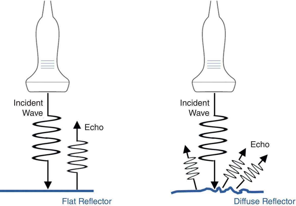
Reflection
Refraction
Scattering
Interface
R
Liver–air
0.9995
Liver–lung
0.684
Liver–bone
0.651
Liver–fat
0.089
Liver–muscle
0.0149
Liver–blood
0.0123 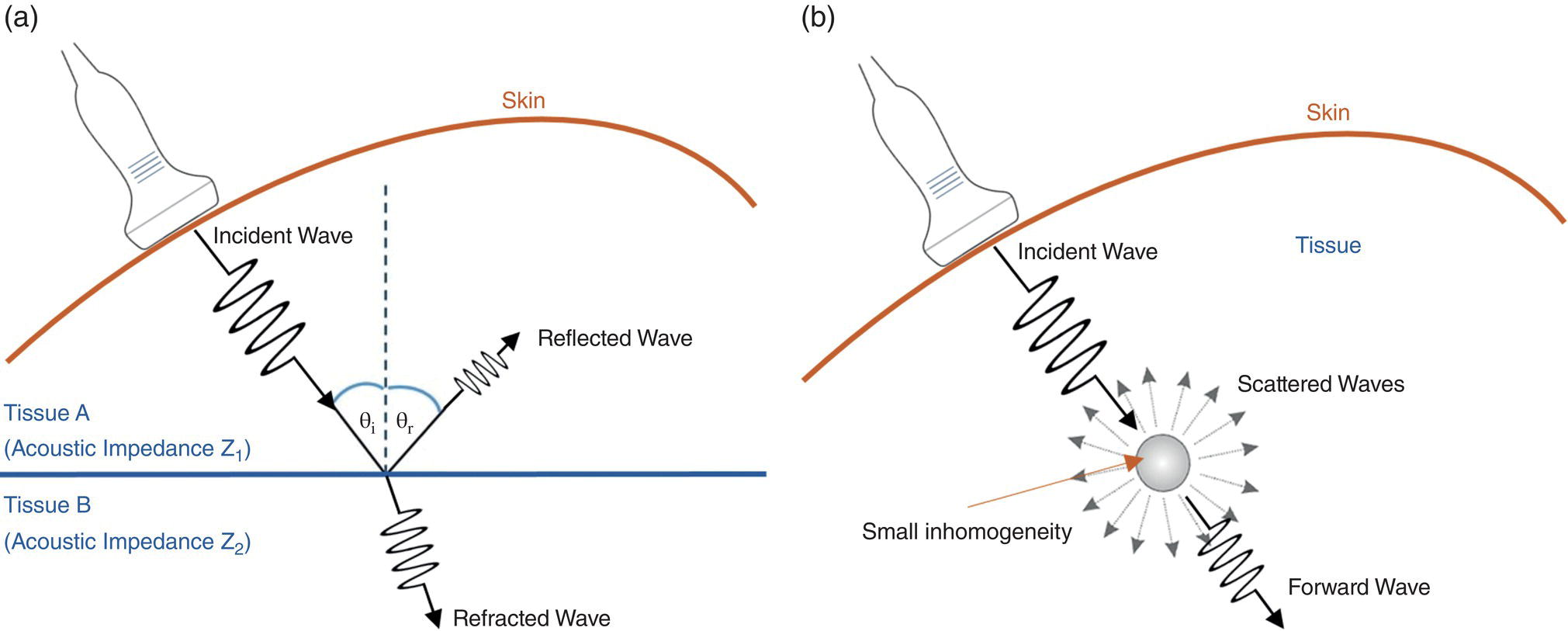
Absorption
Attenuation
Ultrasound Transducers
Piezoelectric Effect
Resonance Frequency
Transducer Bandwidth
Single‐Element Transducer
Imaging with a Single Element
Array Transducers and Transmit Beamforming
Line‐by‐Line Scan
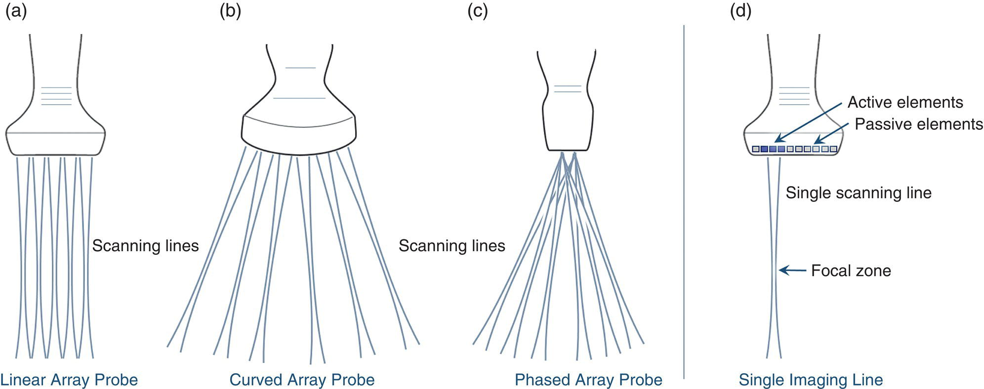
Ultrasound Image Formation
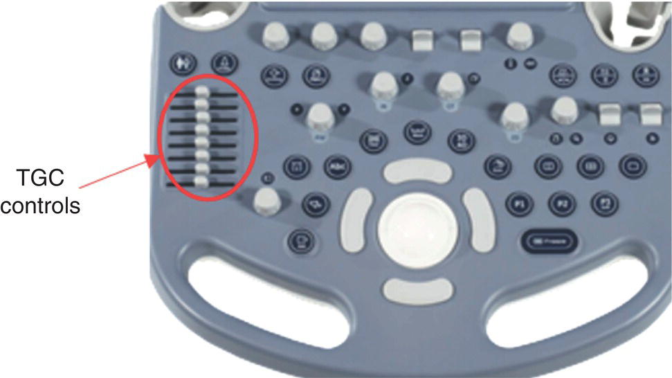
Pre‐processing and Receive Beamforming
Pre‐processing
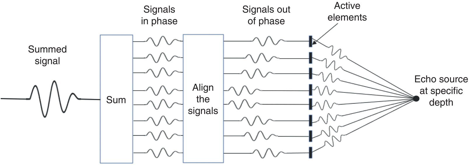
Delay‐and‐Sum Receive Beamforming
B‐Mode Ultrasound
Fundamental Frequency B‐Mode Imaging
Harmonic Imaging
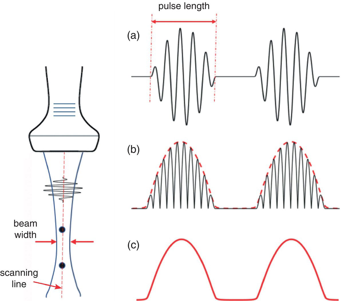
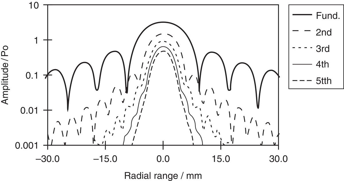
Image Resolutions
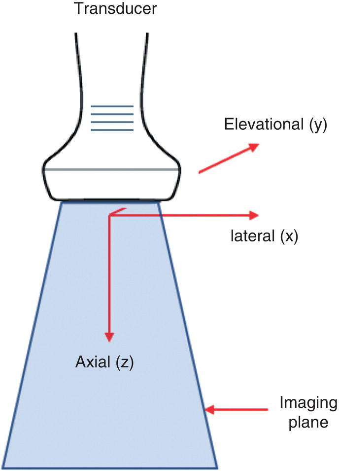
Image Display
Doppler Ultrasound
Doppler Effect


Related posts:

Stay updated, free articles. Join our Telegram channel

Full access? Get Clinical Tree


