Gradient Echo: Part I (Basic Principles)
Introduction
In this chapter, we introduce the gradient-echo (GRE) pulse sequence. It is also called gradientrecalled echo (GRE), the reason for which will become clear later in the chapter. The major purpose behind the GRE technique is a significant reduction in the scan time. Toward this end, small flip angles are employed, which, in turn, allow very short repetition time (TR) values, thus decreasing the scan time. Consequently, such techniques are also referred to as partial flip angle techniques. One of the most important applications of GRE is the ability to employ three-dimensional (3D) imaging, thanks to the higher speed of GRE due to very short TRs. The major differences between GRE and spin-echo (SE) sequences are explained in this chapter.
Gradient-Recalled Echo
As mentioned in the introduction, the purpose of the GRE technique is to increase the speed of the scan. Recall that the scan time for “conventional” techniques is given by
where TR is the repetition time, Ny the number of phase-encoding steps, and NEX the number of excitations. Now, Ny is generally selected to yield a certain resolution (too small an Ny degrades the resolution), and NEX is chosen to yield a certain signal-to-noise ratio (SNR). Consequently, the only parameter in Equation 20-1 that can be controlled to reduce the scan time is TR.
In other words, we wish to select a TR that is as small as possible and still be able to receive a reasonable echo to create an image. If we use 90° radio frequency (RF) pulses, then with very small TRs, the longitudinal magnetization is not given sufficient time to recover to a reasonable value, as depicted in Figure 20-1. This causes a significant reduction in the longitudinal magnetization and the subsequent transverse magnetization (Fig. 20-2). That is, the amplitude of the received signal will be diminished significantly (and, thus, SNR is deteriorated).
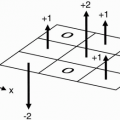
To rectify this problem, an RF pulse yielding a smaller flip angle α is used instead of the usual 90° RF pulse. This change causes incomplete flipping of the longitudinal magnetization into the x-y plane, producing transverse magnetization, called, Mxy (Fig. 20-3). In addition, the major component of magnetization remains along the z-axis after the RF pulse (called Mz). Consequently, even with small TRs, there will be sufficient longitudinal magnetization at the time of the next cycle.
MATH: For the mathematically oriented reader, the magnitude of the transverse and longitudinal magnetizations are given by
right after the α RF pulse, where M0 is the initial magnetization.
After this point, the process of recovery along the z-axis and the process of dephasing in the x-y plane are exactly the same as in its SE counterpart. There is, however, one major difference between GRE and SE sequences. In SE, a 180° refocusing pulse is used to eliminate dephasing
caused by external magnetic field inhomogeneities. This pulse is not used in GRE imaging.
caused by external magnetic field inhomogeneities. This pulse is not used in GRE imaging.
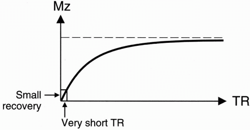 Figure 20-1. After a 90° pulse, longitudinal recovery after a short TR will be very small. |
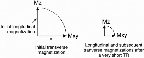 |
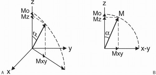 Figure 20-3. A-B: If a small flip angle α is used, only a portion of longitudinal magnetization is flipped into the x-y plane, and thus a portion of longitudinal magnetization will remain. |
 |
Question: What is the reason for not using a 180° refocusing pulse in GRE?
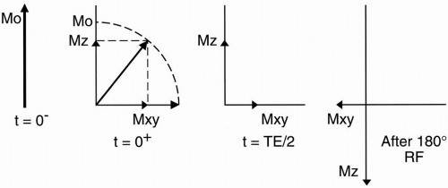
Answer: Because we use a small flip angle in GRE, there would be a large component in the longitudinal axis at half the echo time (TE/2). (In SE imaging, however, this longitudinal component is insignificant at TE/2 because TE/2 is much smaller than T1 of the tissue.) Let’s see what would happen to this longitudinal magnetization if we were to apply a 180° pulse. Although the application of a 180° pulse does yield rephasing in the x-y plane, it also causes Mz to invert and point south (Fig. 20-4). To recover this inverted vector back in the north direction requires a long TR, which is clearly not the desired case in GRE. (The above is not a problem in conventional SE imaging because the longitudinal magnetization at TE/2 is very small and inverting it does not pose any significant loss of signal.)
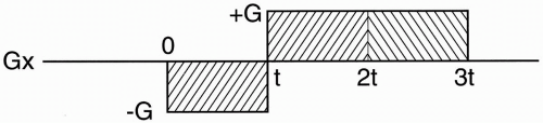 Figure 20-5. Instead of using a 180° pulse, a bilobed gradient is used that has a negative lobe as well as a positive lobe of twice the duration. |
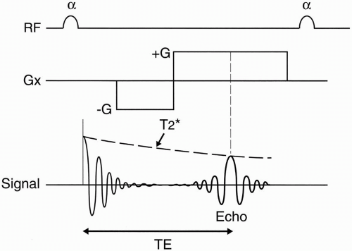
Question: In the absence of a 180° pulse, how does one form an echo?
Answer: One way is to measure the free induction decay (FID) instead. However, it’s impractical to do so because the FID comes on too early and decays more rapidly than we can spatially encode the signal. We need time to apply a phase-encoding gradient and prepare the signal for frequency encoding. We also need time to let the RF pulses and gradients die down before doing anything else. To this end, we will intentionally dephase the FID and rephase (or recall) it at a more convenient time, namely, at TE. This is accomplished via a refocusing gradient in the x direction and is illustrated in Figure 20-5. This gradient has an initial negative lobe that intentionally dephases the spins in the transverse plane and thus eliminates the FID. It is then followed by a positive lobe that rephases the spins, thus restoring the FID in the form of a readable echo. The area under the negative lobe is equal
to half the area under the positive lobe. The refocusing occurs at the midpoint of the positive lobe. Figure 20-6 illustrates how the FID is refocused at TE. In other words, the FID is first eliminated and then recalled at time TE; hence the name gradient-recalled echo.
to half the area under the positive lobe. The refocusing occurs at the midpoint of the positive lobe. Figure 20-6 illustrates how the FID is refocused at TE. In other words, the FID is first eliminated and then recalled at time TE; hence the name gradient-recalled echo.
Slice Excitation
The other difference between GRE and SE is that in GRE imaging, TR may be too short to allow for processing of other slices. For this reason, short TR GRE techniques may acquire only one slice at a time. This is referred to as sequential scanning. (In the next chapter, we will introduce variations of GRE that allow multiplanar imaging by lengthening the TR.) In other words, in a sequential mode (single-slice) GRE, the total scan time is given by
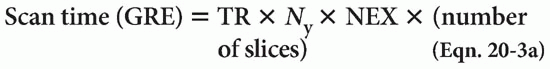
That is to say, acquisition of additional slices increases the scan time in a sequential mode in GRE imaging.
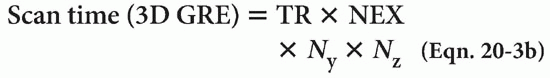
where Ny and Nz refer to the number of phaseencoding steps in the y and z directions, respectively.
Example
Suppose TR = 50 msec, TE = 15 msec, α = 15°, NEX = 1, and Ny = 128. Then TR × NEX × Ny × 50 × 128 × 1 = 6400 msec = 6.4 sec
Thus, it takes only 6.4 sec to obtain a single slice. If we were to obtain 10 slices, the scan time would be Scan time (10 slices) = 6.4 × 10 = 64 sec = 1 min, 4 sec
whereas acquisition of 20 slices would take Scan time (20 slices) = 6.4 × 20 = 128 sec = 2 min, 8 sec
which is twice as long.
Magnetic Susceptibility
The lack of a 180° refocusing pulse results in greater dephasing of spins compared with conventional SE. This in turn results in greater sensitivity to magnetic susceptibility effects. This increased sensitivity can be both problematic (e.g., increased artifact at the air/tissue interfaces) and advantageous (e.g., when searching for subtle hemorrhage), depending on the application (Figs. 20-7 and 20-8).
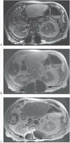 Figure 20-7. Axial T1 gradient echo out of phase (TR 110/TE 2) (A), and T1 gradient echo in phase (TR 110/TE 4) (B) images show marked “blooming” artifact (arrows) from the patient’s known spinal fixation hardware. The out-of-phase image (A) has less artifact than the in phase image (B) due to the shorter TE. Axial T2 FSE (C) and ½ NEX SSFSE T2 |
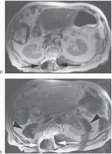 Figure 20-7. (continued) (D) images have less artifact due to multiple 180° refocusing RF pulses with the SSFSE having the least due to the longest echo train length. Finally, an axial T2 FSE image with fat saturation (E) shows ferromagnetic artifact (arrows) and magnetic field changes resulting in paradoxical water saturation (arrowheads) and very poor fat saturation. |
Steady-State Transverse Magnetization
There is one more major difference between GRE and SE pulse sequences. Whereas at the start of each cycle in SE imaging in which there is negligible component of magnetization Mxy in the x-y plane, this may not be the case in GRE imaging. In other words, GRE may have residual transverse magnetization at the end of the cycle, which will be affected by the next RF pulse. This is because in GRE imaging, TR may be too short to allow for complete dephasing (i.e., T2* decay) of the spins in the transverse plane. (In contrast, in SE imaging, TR is long enough to allow complete dephasing of the spins in the x-y plane.) After a few cycles, this residual transverse magnetization reaches a steady state, referred to as Mss. This scheme is illustrated in Figure 20-9 and is elaborated upon further in the next chapter.
Tissue Contrast
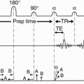
Figure 20-10 depicts a generic GRE pulse sequence diagram (PSD). There are three operatorcontrolled parameters that affect the tissue contrast: α, TR, and TE. Let’s discuss how each of these plays a role in this matter.
First, consider a small flip angle α (e.g., 5° to 30°). As can be seen in Figure 20-11, a small flip angle results in a large amount of (persistent) longitudinal magnetization after application of the RF


Related posts:
Stay updated, free articles. Join our Telegram channel
Full access? Get Clinical Tree
