Image Reconstruction

(1)

Cleveland Clinic, Emeritus Staff, Cleveland, OH, USA

Keywords

Image reconstructionFiltered backprojectionIterative methodsMLEMOSEMPartial volume

Introduction

Projection data acquired in two-dimensional (2D) mode or three-dimensional (3D) mode are stored in sinograms that consist of rows and columns representing angular and radial samplings, respectively. Acquired data in each row are compressed (summed) along the depth of the object and must be unfolded to provide information along this direction. Such unfolding is performed by reconstruction of images using acquired data. The 3D data are somewhat more complex than the 2D data and usually rebinned into 2D format for reconstruction. After correction for the factors discussed in Chap. 3, the data are used to reconstruct transaxial (transverse) images from which vertical long axis (coronal) and horizontal long axis (sagittal) images are formed. Reconstruction of images is made by two methods: filtered backprojection and iterative methods. Both methods are described below.

Simple Backprojection

In 2D acquisition, activity in a given line of response (LOR) in a sinogram is the sum of all activities detected by a detector pair along the line through the depth of the object. The principle of backprojection is employed to reconstruct the images from these acquired LORs. A reconstruction matrix of a definite size (e.g., 128 × 128 pixels) is chosen. While the image matrix is in (X, Y) coordinates, the sinogram data are in polar coordinates. An image pixel at (X, Y) position is related to polar coordinates (r, ϕ) (Fig. 3.3a) by

$r=x\; \sin\;\phi +y \cos\;\phi .$

(4.1)

For each image pixel (X, Y) at each projection angle ϕ, r is calculated by Eq. (4.1). The measured counts in the projection sinogram corresponding to the calculated r are added to the (X, Y) pixel in the reconstruction matrix. This is repeated for all projection angles. Thus, the backprojected image pixel f(X, Y) in the reconstruction matrix is given by

$f\left(X,Y\right)=\frac{1}{N}{\displaystyle {\sum}_{N=1}^Np\left(r,\phi \right)}$

(4.2)

where p(r, ϕ) is the count density in the sinogram element in the acquired matrix and N is the number of projection angles. When all pixels are computed, a reconstructed image results from this simple backprojection (Fig. 4.1).

Fig. 4.1

Principle of backprojection in image reconstruction. (a) An object with two hot spots (solid spheres) is viewed at three projection angles (at 120° angle) and the acquired data are backprojected for image reconstruction; (b) when many views are obtained, the reconstructed image represents the activity distribution with “hot” spots, but the activity is blurred around the spots; (c) blurring effect described by a 1/r function, where r is the distance away from the central point (Reprinted with the permission of The Cleveland Clinic Center for Medical Art & Photography ^©2009. All Rights Reserved)

In another approach of simple backprojection, in the reconstruction matrix of chosen size, the counts along an LOR in a sinogram detected by a detector pair are projected back along the line from which they originated. The process is repeated for all LORs, i.e., for all detector pairs in the PET scanner. Thus, the counts from each subsequent LOR are added to the counts of the preceding backprojected data, resulting in a backprojected image of the original object.

Filtered Backprojection

The simple backprojection has the problem of “star pattern” artifacts (Fig. 4.1a) caused by “shining through” radiations from adjacent areas of increased radioactivity resulting in the blurring of the object (Fig. 4.1b). Since the blurring effect decreases with distance (r) from the object of interest, it can be described by a 1/r function (Fig. 4.1c). It can be considered as a spillover of some counts from a pixel of interest to the neighboring pixels, and the spillover decreases from the nearest pixels to the farthest pixels of different frequencies. The blurring effect is minimized by applying a filter to the acquisition data, and filtered projection data are then backprojected to produce an image that is more representative of the original object. Such methods are called the filtered backprojection and are accomplished by the Fourier method described below.

The Fourier Method

According to the Fourier method, the measured line integral p(r, ϕ) in a sinogram is related to the count density distribution f(X, Y) in the object obtained by the Fourier transformation. The projection data obtained in the spatial domain (Fig. 4.2a) can be expressed in terms of a Fourier series in the frequency domain as the sum of a series of sinusoidal waves of different amplitudes, spatial frequencies, and phase shifts running across the image (Fig. 4.2b). This is equivalent to sound waves that are composed of many sound frequencies. The data in each row of an acquisition matrix can be considered to be composed of sinusoidal waves of varying amplitudes and frequencies in the frequency domain. This conversion of data from spatial domain to frequency domain is called the Fourier transformation (Fig. 4.3). Similarly the reverse operation of converting the data from frequency domain to spatial domain is termed the inverse Fourier transformation.

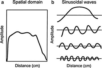
Fig. 4.2

Representation of data in the spatial and frequency domains. The activity distribution as a function of distance in an object (spatial domain) (a) can be expressed as the sum of the four sinusoidal functions (b)

Fig. 4.3

The Fourier transform of this activity distribution is represented, in which the amplitude of each sine wave is plotted at the corresponding frequency of the sine wave

In the Fourier method of backprojection, the projection data in each profile are subjected to the Fourier transformation from spatial domain to frequency domain, which is symbolically expressed as

$F\left({\nu}_x{\nu}_y\right)=\mathcal{F}\dot{c}f\left(X,Y\right),$

(4.3)

where F(ν _x, ν _y) is the Fourier transform of f(X, Y) and $\mathcal{F}$ denotes the Fourier transformation. In essence, the Fourier transform F(ν _x, ν _y) of each projection in the sinogram of the 2D projection data is taken prior to backprojection. Straight backprojection of these Fourier projections produces a blurred image because of the oversampling at the center and less sampling at the edge. To reduce blurring (i.e., to improve the signal-to-noise ratio), the Fourier projections must be “filtered” using appropriate filters.

A filter, H(ν), in the frequency domain is applied to each projection, i.e.,

${F}^{\prime}\left(\nu \right)=H\left(\nu \right)\cdot F\left(\nu \right),$

(4.4)

where F′(ν) is the filtered Fourier projection which is obtained as the product of H(ν) and F(ν).

Finally, the inverse Fourier transformation is performed to obtain filtered projection data in the spatial domain, which are then backprojected in the same manner as in the simple backprojection. With the use of faster computers, the Fourier technique of filtered backprojection has gained wide acceptance in reconstruction of images in nuclear medicine.

Several factors affect the filtered backprojection. Adequate sampling of projections (both linear and angular projections related to r and ϕ of the sinogram) is needed for accurate backprojection. Data noise, positron range, noncolinearity, scattering, and random events are not taken into consideration in the method. Also in this model, detectors are assumed to be point sources, whereas in reality they have dimensions that cause nonuniform distribution of activity resulting in nonuniform projection.

Types of Filters

A number of Fourier filters have been designed and used in the reconstruction of tomographic images in nuclear medicine. All of them are characterized by a maximum frequency, called the Nyquist frequency, which gives an upper limit to the number of frequencies necessary to describe the sine or cosine curves representing an image projection. Because the acquisition data are discrete, the maximum number of peaks possible in a projection would be in a situation in which peaks and valleys occur in every alternate pixel, i.e., one cycle per two pixels or 0.5 cycle/pixel, which is the Nyquist frequency. If the pixel size is known for a given matrix, then the Nyquist frequency can be determined. For example, if the pixel size in a 64 × 64 matrix is 4.5 mm for a given detector, then the Nyquist frequency will be

$\begin{array}{c}\mathrm{Nyquist}\ \mathrm{frequency}=0.5\;\mathrm{cycle}/\mathrm{pixel}\\ {}=0.5\;\mathrm{cycle}/0.45\;\mathrm{cm}\\ {}=1.11\;\mathrm{cycle}/\mathrm{cm}.\end{array}$

A common well-known filter is the ramp filter (name derived from its shape in the frequency domain) shown in Fig. 4.4 in the frequency domain. An undesirable characteristic of the ramp filter is that it amplifies the noise associated with high frequencies in the image even though it removes the blurring effect of simple backprojection. To eliminate the high-frequency noise, various filters have been designed by including a window in them. Such filters are basically the products of the ramp filter with a sharp cutoff at the Nyquist frequency (0.5 cycle/pixel) and a window with amplitude 1.0 at low frequencies but gradually decreasing at higher frequencies. A few of these windows (named after those who introduced them) are illustrated in Fig. 4.5, and the corresponding filters (more appropriately, filter–window combinations) are shown in Fig. 4.6.

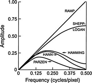
Fig. 4.4

The typical ramp filter in the frequency domain

Fig. 4.5

Different windows that are used in combination with a ramp filter to suppress the higher frequency noise in backprojection method

Fig. 4.6

Different filters (filter–window combinations) that are obtained by multiplying the respective windows by the ramp filter with cutoff at Nyquist frequency of 0.5 cycle/pixel

The effect of a decreasing window at higher frequencies is to eliminate the noise associated with the images. The frequency above which the noise is eliminated is called the cutoff frequency (ν _c). As the cutoff frequency is increased, spatial resolution improves and more image detail can be seen up to a certain frequency. At a too high cutoff value, image detail may be lost due to inclusion of inherent noise. Thus, a filter with an optimum cutoff value should be chosen so that primarily noise is removed, while image detail is preserved. Filters are selected based on the amplitude and frequency of noise in the data. Normally, a filter with a lower cutoff value is chosen for noisier data as in the case of obese patients and in ²⁰¹Tl myocardial perfusion studies or other studies with poor count density.

Hann, Hamming, Parzen, and Shepp–Logan filters are all “low-pass” filters, because they preserve low-frequency structures while eliminating high-frequency noise. All of them are defined by a fixed formula with a user-selected cutoff frequency (ν _c). It is clear from Fig. 4.6 that while the most smoothing is provided by the Parzen filter, the Shepp–Logan filter produces the least smoothing.

An important low-pass filter that is most commonly used in nuclear medicine is the Butterworth filter (Fig. 4.7). This filter has two parameters: the critical frequency (f _c) and the order or power (n). The critical frequency is the frequency at which the filter attenuates the amplitude by 0.707, but not the frequency at which it is reduced to zero as with other filters. The parameter, order n, determines how rapidly the attenuation of amplitudes occurs with increasing frequencies. The higher the order, the sharper the fall. Lowering the critical frequency, while maintaining the order, results in more smoothing of the image.