Introduction
In medical imaging, a three-dimensional (3D) image, or volume, is often acquired by stacking up a series of two-dimensional (2D) slice images. Just as 2D images are made up of pixels, 3D volumes such as computed tomography (CT) or magnetic resonance imaging (MRI) scans consist of voxels as the basic elements. The printing of a specific object (bone, tissue, etc.) from a medical image usually involves the following steps ( Fig. 3.1 ):
- 1.
The raw volumetric image dataset containing the target object is acquired.
- 2.
Voxels belonging to the target object are marked on the stack of 3D images.
- 3.
A 3D surface is reconstructed from the cluster of voxels forming the target object.
- 4.
The 3D surface is smoothed and fixed for any topological defects.
- 5.
The polished 3D surface is exported for printing.

The procedure of marking a target object on an image is known as segmentation. Segmentation can be performed manually slice by slice on the image stack, using software with a paintbrush or a lasso tool. However, this approach can be extremely time-consuming, as modern medical images often contain hundreds of slices. One way to accelerate the procedure is to perform manual segmentation only on selected slices (e.g., alternate slices or every third slice), with interpolation in between. Some software packages, such as Mimics (Materialise, Leuven, Belgium), support 3D interpolation between orthogonal slices (axial, coronal, or sagittal). However, when processing a large number of medical images, manual segmentation is still limited in efficiency and consistency. To solve this problem, various automated segmentation algorithms have been developed.
Most automated segmentation algorithms rely on the signal intensity of voxels (abbreviated as voxel intensities, or just intensities). The voxel intensities not only reflect the characteristics of the imaged tissue (e.g., proton density in MRI, radiodensity in CT) but are also affected by the setup parameters of the scanner (e.g., echo time and repetition time in MRI). In general, the image segmentation algorithms can be categorized into region-based (3.1.1), boundary-based (3.1.2), atlas-based (3.1.3), and classification-based (3.1.4). Accurate segmentation of medical images often depends on the intensity features of the target object, or the intensity difference between target and background. However, undesirable artifacts may be introduced during the imaging procedure, such as noise, nonuniformity, partial volume effect, etc. These artifacts may cause geometric distortion and missegmentation of the target object. Therefore, preprocessing is often necessary in order to improve the segmentation accuracy (see Section Nonuniformity Correction for Accurate MRI Segmentation ).
Region-Based Segmentation
In region-based segmentation, the algorithms are based on the intensity homogeneity within the target object and/or the background. The simplest example of a region-based algorithm is intensity thresholding, where the input 3D image is divided into foreground (i.e., target object) and background, by comparing the intensity of each voxel to a constant value (threshold). The output of thresholding is usually a binary image of the same dimension as the input image, called a mask. Let I(x , y , z) be the voxel intensity at coordinate (x , y , z) , then the voxel intensity of mask M is defined as
M(x,y,z)={0ifI(x,y,z)<T1otherwise
Another commonly used region-based algorithm is region growing. First, a seed region containing one or more voxels is defined on the 3D image, either manually or by automated computational tools. The seed region is then extended to its neighboring voxels, until it reaches certain preset constraints, such as the similarity of all neighbors. The final form of the region is used as the target object. A common example of region growing is the watershed algorithm. Consider a simple case of a 2D image. The image is treated as an elevation map, with voxel intensity representing the voxel’s altitude. The watershed method uses one of two strategies to decompose the image into subregions, or watersheds: 1) flooding or immersion and 2) rainfall. For both strategies, the process begins with identifying and tagging all local minima. In watershed by flooding, water sources are placed in each local minimum. The water level is systematically increased, creating a set of barriers. The process terminates when different water regions merge. In watershed by rainfall, for each voxel, the algorithm finds the direction in which a raindrop would flow if it fell on this voxel. The neighboring voxel is found at the flow direction. The voxel and its neighbor are then merged, and the process continues until the local minimum is reached.
Instead of region growing, sometimes region peeling is necessary in order to reduce the size of the segmented region, or separate two target regions touching each other. The mathematical morphology provides an elegant framework for both region growing and region peeling. For binary morphology, a binary mask (named a structuring element) B is set, which defines the connected components (or neighborhood) for any voxel z in the image. Common 2D examples of B are illustrated in Fig. 3.2 . Note that the radius of B is conventionally an odd number. The 3D version of B can be obtained by extending the 5 × 5 matrices in Fig. 3.2 to 5 × 5 × 5 matrices, while maintaining the same binary profiles.

Let A be the input image. Then for any given voxel z in A, a set of connected voxels (denoted B z ) can be obtained by shifting the center of the structuring element B to the coordinates of z and including all the voxels covered by B. The four basic morphological operations —erosion E(A , B) , dilation D(A , B) , opening O(A , B) , and closing C(A , B) — can then be defined as
E(A,B)={z|Bz⊆A}D(A,B)={z|Bz∩A≠∅}C(A,B)=E(D(A,B),B)O(A,B)=D(E(A,B),B)
In other words, the erosion of image A by element B is the set of all voxels z such that B z is contained in A , while the dilation of A by B is the set of all voxels z such that B z overlaps with A by at least one voxel. The closing operation, which consists of dilation followed by erosion, is particularly useful for 3D printing, as it can fill small holes in the segmented regions before 3D reconstruction and printing.
In practice, different region-based algorithms can be combined to achieve more accurate segmentation. For example, in orthopedic imaging, thresholding and morphological operations can be jointly applied to separate gypsum cast from the bone on CT scans ( Fig. 3.3 ).

Boundary-Based Segmentation
In boundary-based segmentation, the algorithms locate the tissue boundary (i.e., the edge) by evaluating local changes (known as gradients) of voxel intensity. For example, the Canny edge detector measures the intensity gradient within a moving window called a kernel. The active contours algorithm converts intensity change into the energy functions, and locates the boundary via optimization searches.
A boundary-based algorithm can also be combined with other algorithm types to achieve a more sophisticated segmentation. One such example is the EdgeWave algorithm in FireVoxel , which combines boundary detection with thresholding and morphology, or the shape characteristics of an image ( Fig. 3.4 ). In FireVoxel, the EdgeWave algorithm is used for several key processing workflows, such as measuring body fat composition on abdominal CT images. The EdgeWave algorithm contains the following main steps:
- 1.
The original image is resampled, as needed.
- 2.
Thresholding by image intensity is applied to roughly delineate the region that needs to be segmented, called the Core Set. The Core Set must enclose the segmentation target, otherwise the segmentation will fail.
- 3.
Edges detection is performed and the locations of the Core Set where image intensity changes abruptly are defined.
- 4.
The boundary of the Core Set is eroded, or peeled. The Peel operation removes all voxels within a certain distance from the boundary using rules applied to each voxel and its neighbors. Peeling enlarges the gaps between different regions of the image, removes small details, and breaks “bridges” between weakly connected areas. The thickness of the region to be removed is controlled by the peel distance , measured in voxels or millimeters.
- 5.
The algorithm breaks up the peeled Core Set into blobs, or connected components. It then determines which connected components are to be retained and which ones should be discarded.
- 6.
The selected connected components are subjected to constrained growth, or dilation. The Grow operation adds voxels within a given distance of the region of interest (ROI) boundary. Any recovered voxels must still belong to the Core Set. The thickness of the recovered region is controlled by the grow distance , which should be larger than the peel distance .

Atlas-Based Segmentation
In atlas-based segmentation, ROIs are first segmented (usually manually) on a reference image called a template. This reference segmentation is commonly known as the atlas. To perform segmentation on a new image, the template image is first warped to the target image through image registration. The same transformation computed during the registration step is then applied to the preexisting atlas to propagate the ROIs on the target image. Fig. 3.5 illustrates this procedure with brain image samples. To reduce the impact of intersubject variability, multiple reference images can be registered to the same target image, with different reference segmentations propagated and merged into a final segmentation. This approach is called multi-atlas segmentation.

Classification-Based Segmentation
In classification-based algorithms, the segmentation is achieved by classifying certain image features. Classifications can be grouped into supervised and unsupervised types. Unsupervised classifications, such as K-means clustering, are achieved without prelabeled training data. Supervised classifications, on the other hand, rely on prior knowledge of target objects imported from the training dataset. For example, the Markov random field algorithm treats the segmentation labels as random variables with a certain probability distribution, where conditional probabilities and the Bayesian theorem relate class probabilities and voxel values. A new family of classification methods has emerged from the recent developments in deep learning, based on convolutional neural network (CNN) models. In CNN models, raw intensity features derived from the image go through successive layers of processing to become high-level abstract features, before weighing into the final classification. One of the most successful CNN models in biomedical image segmentation is the U-net model, whose layers consist of downsampling followed by upsampling (thus forming a U-shape model architecture).
Nonuniformity Correction for Accurate MRI Segmentation
Image intensity nonuniformity is a common MRI artifact, manifested by the variation of signal intensity across the image even within the same tissue. This artifact is also referred to as shading, bias field, or image inhomogeneity. Nonuniformity may be caused by RF field inhomogeneity, inhomogeneous receiver coil sensitivity, and patient’s influence on the magnetic and electric fields. While smoothly varying nonuniformity does not appear to affect visual radiologic diagnosis, it is detrimental to tissue quantification, including image segmentation. Medical image segmentation methods require that a given tissue be represented by constant signal intensity throughout the field of view. Thus, correcting for nonuniformity artifact is a crucial step. Several nonuniformity correction approaches have been developed for a variety of applications.
Prospective Approaches
Prospective nonuniformity correction methods acquire information to infer the spatial pattern of nonuniformity. The earliest attempts, inspired by the methods employed to calibrate scintillation detectors in nuclear medicine, used images of a uniform phantom acquired using the same sequence as the one used for patient imaging. Such efforts have been mostly abandoned due to the realization that this approach ignores the significant influence of the electromagnetic properties of the object being imaged and their interaction with magnetic field.
More recent methods acquire additional calibration information by imaging the patient using different sequences. Their goal is to estimate the sources of the nonuniformity artifact, such as the flip angle variation. An important example of this approach is the MP2RAGE sequence, which aims to improve on a well-known MPRAGE (Magnetization-Prepared RApid Gradient Echo) sequence. Developed in the early 1990s, MPRAGE remains the most popular sequence for high-resolution T1-weighted brain imaging. The sequence begins with a nonselective 180-degree inversion pulse that inverts the magnetization. The magnetization then recovers over an inversion time interval (TI), which is typically 700–1000 ms at 3T. This recovery interval is followed by a series of gradient echo samplings characterized by a short (about 3 ms) echo time and small (about 10 degree) flip angles.
MPRAGE images are often corrupted by gradient field inhomogeneities, susceptibility, and eddy current effects. The MP2RAGE sequence has been developed to correct for these shortcomings. MP2RAGE introduces a second inversion time, TI2 (with the typical value of 2500 ms at 3T), in order to acquire a second readout with predominantly spin density-weighted contrast. By combining image data from the first and second readouts, the T2∗ and B1 inhomogeneity effects can be largely canceled out, generating a new and more uniform T1-weighted image at the cost of a longer acquisition time ( Fig. 3.6 ).