Medical imaging technologies, which allow us to “see into” and understand living systems, play a significant role in biology and medicine. The X-ray has paved the way for many high-tech medical imaging technologies that are used today including computed tomography (CT), magnetic resonance imaging (MRI), ultrasound, and positron emission tomography (PET). It is possible a number of scientists inadvertently produced X-rays including William Morgan and Nicola Tesla. However, the real discovery and understanding of the X-ray was by Wilhelm Röntgen in late 1895 when he realized X-rays could pass through opaque objects and could be used to generate an image. Röntgen was the first to document this phenomenon using a recording of a photograph of the bones in his wife’s hand, and he coined the term “X-ray.”
X-rays are a penetrating form of electromagnetic radiation carried by photons, with a wavelength ranging from 0.01 to 10 nm that places them into an ionizing radiation category. They are produced in an X-ray tube when a beam of high-energy electrons strikes a high-density target, resulting in production of energy in the form of both heat and these high-energy photons. X-rays have a shorter wavelength and higher frequency than that of visible light.
Not long after X-rays were discovered, the first use of X-rays under clinical conditions was by John Hall-Edwards in Birmingham, England, in 1896 when he radiographed a needle stuck in the hand of an associate. On February 5, 1896, J. T. Bottomley, Lord Blythswood, and John Macintyre gave a presentation to the Philosophical Society of Glasgow on X-rays. Soon after, in March 1896, Mcintyre obtained the permission of the managers of Glasgow Royal Infirmary to set up an X-ray department, which was the first one to be established in the world.
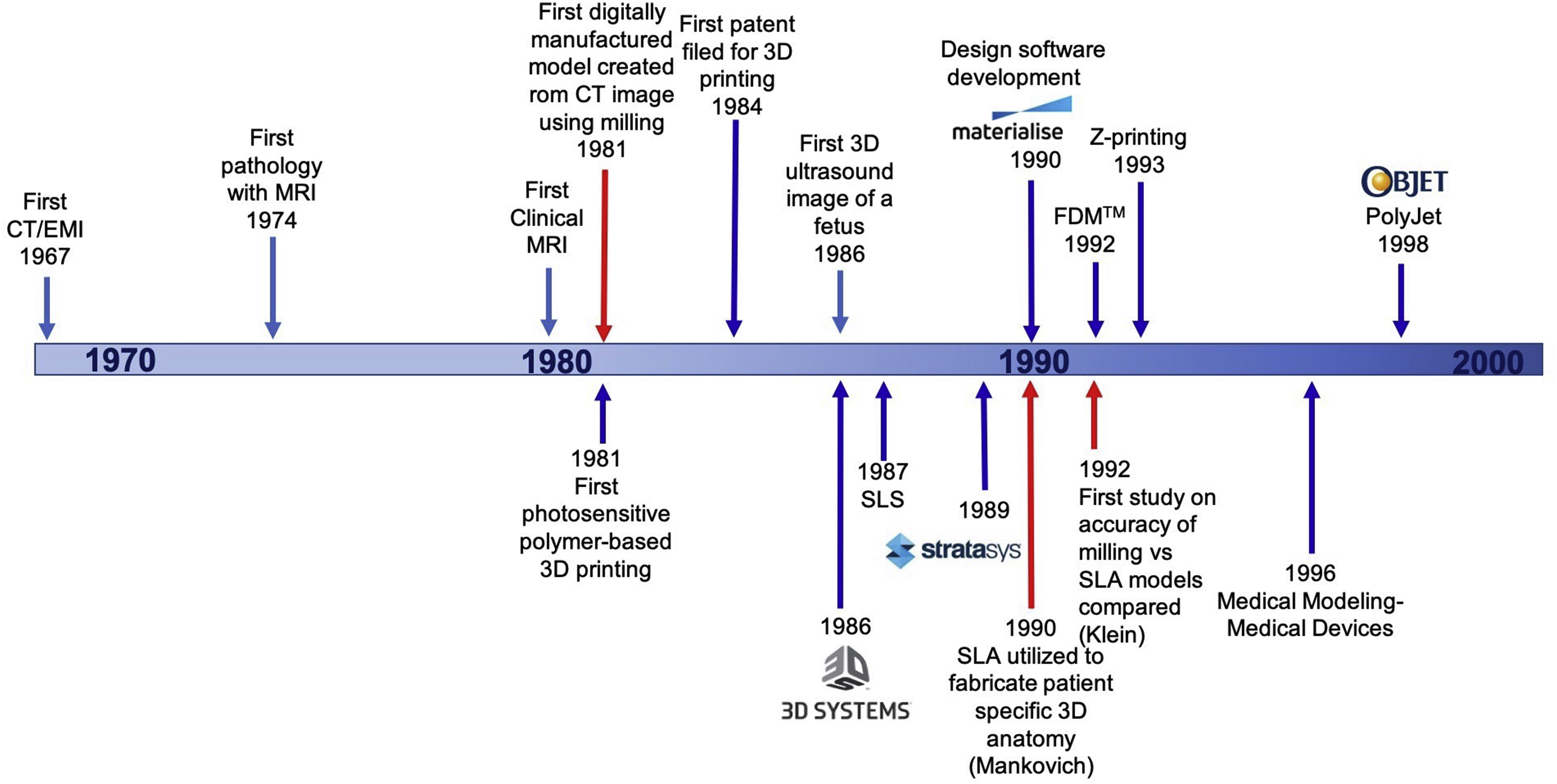
Since the development of the X-ray, there have been many major advancements in medical imaging, and the use of volumetric medical imaging including CT and MRI have played a critical role in the development of medical 3D printing over the years with advancements in both fields being closely intertwined over the decades ( Fig. 2.1 ).
Today, volumetric medical imaging is the backbone of 3D printing in medicine since imaging data are used to create patient-specific, 3D printed anatomic models and guides. Anatomic models may be created from any volumetric dataset, with sufficient contrast and spatial resolution to separate structures, using dedicated image post-processing software (discussed in Chapter 3). When a 3D model is requested prior to an imaging study, the image acquisition and reconstruction techniques should be tailored so that the anatomy in the intended 3D model can be effectively visualized, with the optimal imaging modality, imaging protocol, and image reconstruction depending on the anatomy being imaged.
CT is the most common clinical technique adopted to generate 3D printed anatomic models due to the fact that CT uses X-rays; accordingly, there is only one contrast mechanism, making image post-processing of CT data relatively simple. MRI, which provides exquisite soft tissue contrast without using ionizing radiation, and 3D ultrasound data may also be used. However, implementation is challenging and time-consuming for MRI (due in part to intrinsically low signal-to-noise ratio (SNR) and image artifacts resulting in nonanatomical signal variation); and implementation is even more difficult for ultrasound data due to the non-tomographic nature of ultrasound acquisition. This chapter will review the imaging systems that are typically used to create 3D printed anatomic models including CT, MRI, and ultrasound. Nuclear medicine imaging modalities and utilization of 3D printing will be discussed in Chapter 12.
Computed Tomography
The history of CT dates back to 1917 with the invention of the Radon transform by Johann Radon, an Austrian mathematician, who showed that a function could be reconstructed from an infinite set of its projections. A comprehensive review of the mathematics is available in many texts including Epstein et al. In short, the transformation that takes one-dimensional (1D) projections of a two-dimensional (2D) object over many angles is called the 2D Radon transform. For a fixed angle theta (q) , g(l,q) , is called a projection; and for all l and q , g(l,q) , is the 2D Radon transform of f(x,y) . In order to represent an image, the Radon transform takes multiple, parallel-beam projections of an image from different angles by rotating the source around the center of an image at a specified rotation angle.
Rθ(x’)=∫-∞∞f(x’cosθ-y’sinθ,x’sinθ+y’cosθ)dy’wherex’y’=cosθsinθ-sinθcosθxy
The projection of an object results from the tomographic measurement process at any given angle, θ , and is made up of a set of line integrals ( Fig. 2.2 ). The set of projections of a single slice is called a sinogram.
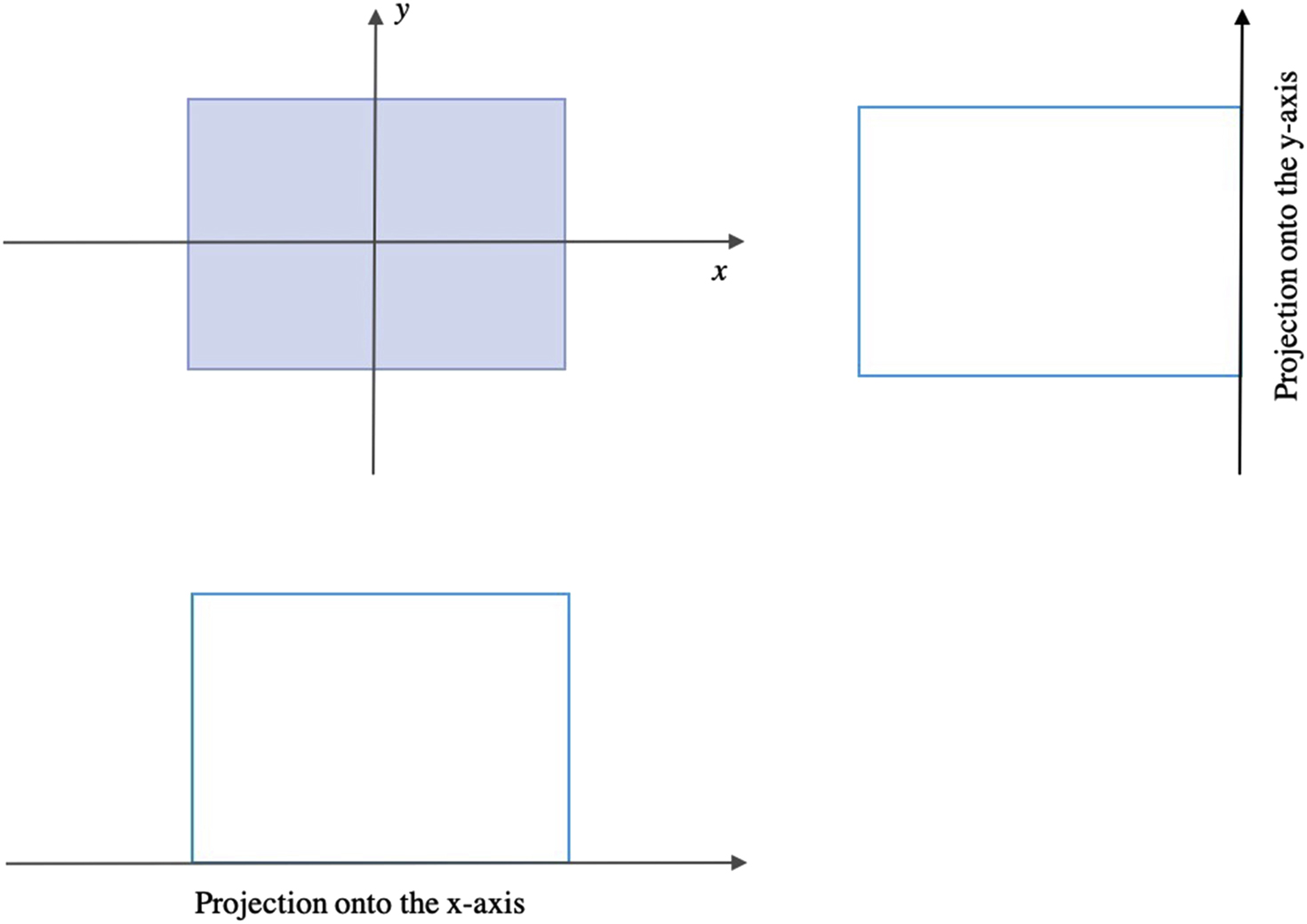
In general, the Radon transform of f(x,y) is the line integral of f parallel to the y’-axis:
The first CT scanner was created in 1967 by Sir Godfrey Hounsfield who, while working at Electrical and Musical Industries (EMI) Central Research Laboratories, used X-rays applied at various angles to create an image of an object. Hounsfield was working on the pattern recognition of letters and was trying to reconstruct a 3D representation of the contents of a box when he realized that it was easier to reconstruct the volume by considering it as a series of slices. Once Hounsfield had verified this principle, he proceeded to construct a testing rig built on the bed of an old lathe that he had from a prior project. This test unit, now known as the “Lathe bed model,” used Americium 95 as its gamma source and had a photon counter as the detector. Initially, it took 9 days to acquire the images and 2.5 h to reconstruct them with an International Computers Limited mainframe computer system.
The first EMI CT scanner was installed in 1971 at the Atkinson Morley Hospital in England and the first human patient brain exam was performed. CT scanners were introduced in the United States (US) a couple of years later with the first clinical scan performed at the Mayo Clinic in 1973. In 1975, EMI marketed the first body scanner which was inaugurally installed at Northwick Park Hospital in London. Shortly after, the first body scanner in the US was installed at the Mallinckrodt Institute at the Washington University School of Medicine in St. Louis, Missouri. By 1976, approximately 17 distinct companies were offering CT scanners and over 475 were sold worldwide. In 1979, Sir Godfrey Hounsfield and Allan McLeod Cormack were both awarded the Nobel Prize in medicine for their pioneering work in the development of CT.
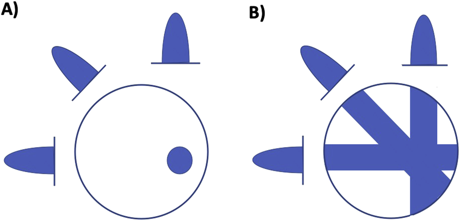
The standard method of reconstructing CT slices is the “backprojection” method which originates from the fact that a 1D projection needs to be filtered by a 1D Radon kernel (backprojected) in order to obtain a 2D signal. The backprojection method starts from a projection value and backprojects a ray of equal pixel values that would sum to the same value ( Fig. 2.3 ). Structures in a complete image can only be restored if a sufficient number of projection angles are collected; however, blurring of the computed image can result if this relatively simple method is employed. Therefore, it is more common to use a filtered backprojection method where a stabilized and discretized version of the inverse Radon transform is typically used.
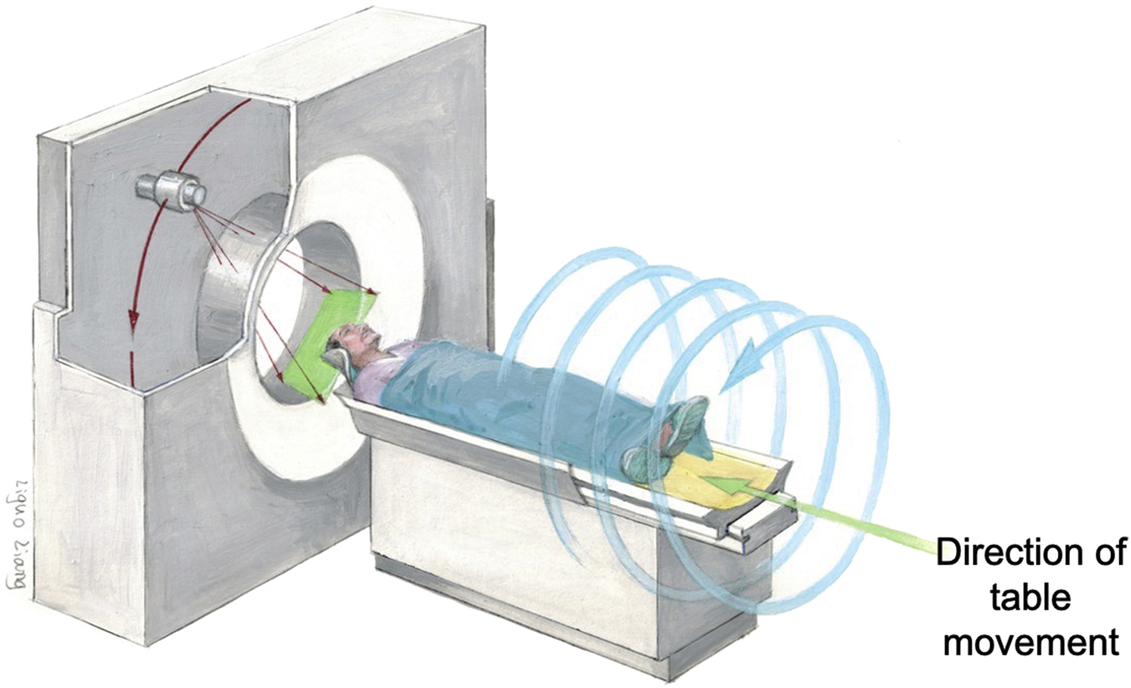
Since the invention of CT, there have been substantial improvements in speed, slice count, radiation dose, and image quality. The important phases in CT development are single-slice CT, helical CT, multiple detector row CT (MDCT) also known as multislice CT, and spectral CT imaging. Single-slice CT systems have 1D detector arrays, thereby acquiring data in a single section plane and reconstructing only one plane per rotation. Helical CT systems perform acquisitions by continually rotating the source and detectors around the patient as the table is moved along the axis of the scanner, enabling the scan to be performed rapidly ( Fig. 2.4 ). The speed of the table is important for exams such as CT angiography where table motions oscillate at several cm/second.
MDCT, introduced in 1992, combines multiple rows of detectors and fast gantry rotation speeds to rapidly gather a cone of X-ray data. MDCT scanners have rapidly evolved from four detector row systems ( Fig. 2.5 ) to systems with 256-slice and 320 detector rows. In comparison to single-row detector CT, MDCT scanners have the advantages of shorter scan durations, longer scan ranges, and thinner slice sections which are especially useful for 3D rendering.
Spectral CT imaging uses different energy levels to capture images, which allows elements in the body to be differentiated based on their material density or atomic number. The energy of the reconstructed image can be altered on a sliding scale and can be processed to create many advantages over conventional CT such as the creation of virtual unenhanced images and amplification/removal of iodine or calcium suppressed images. A comprehensive review by Erik Fredenberg lists the many advantages of this acquisition type including improved soft-tissue and contrast agent–based contrast-to-noise ratio (CNR) and better detection of lesions and plaque characterization.
Cone beam computed tomography (or CBCT), a variant type of CT, uses a cone-shaped X-ray beam and 2D detectors instead of a fan-shaped X-ray beam and 1D detectors. CBCT is important in the field of oral and maxillofacial surgery due to the advantages over conventional 2D X-ray methods, such as ease of imaging in a seated or standing position with a rotation of the gantry around the head. With the availability of the equipment in dentist offices, this method is also used in orthodontics and endodontics. Additionally, image-guided radiation therapy often utilizes this method.
CT images are comprised of grayscale pixels, also known as picture elements. The physical size of a pixel depends on the image resolution which is set in the image acquisition. Similar to a pixel, a voxel represents an array of elements of a volume that constitute a 3D image. Both pixels and voxels typically do not have their position/coordinates explicitly encoded with their values. Instead, rendering systems infer the position of pixels and voxels based on their position relative to other pixels/voxels.
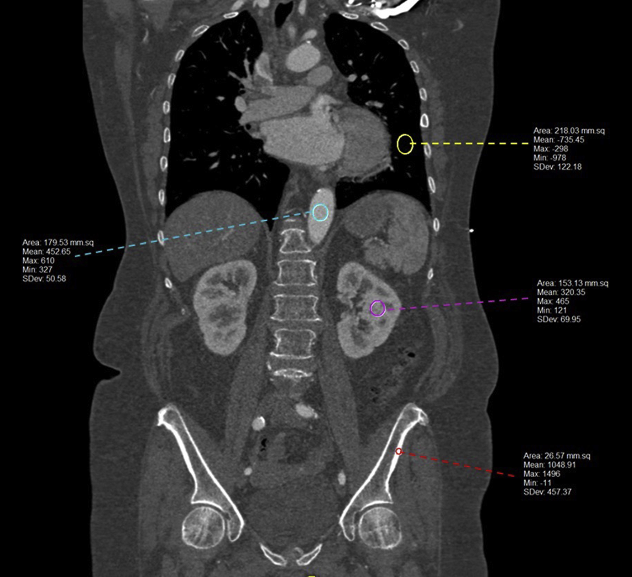
In CT, there is only one contrast mechanism; the grayscale intensity of the image is proportional to the tissue density with the grayscale value seen in each pixel reflecting how the amount of the X-ray beam the tissue attenuated as it passed through the patient. The Hounsfield unit (HU) scale, named after Sir Godfrey N. Hounsfield, used in these images is a linear transformation of the original linear attenuation coefficient mechanism, and it provides information regarding what type of tissue types may be present (i.e., air, bone, soft tissue, blood, etc.). On the HU scale, air is represented by a value of −1000 and appears black on the grayscale image and bone is +1000 and appears white on the grayscale image ( Fig. 2.6 ).
Magnetic Resonance Imaging
MRI is a dynamic and flexible noninvasive imaging technology that operates at the radiofrequency (RF) range and produces detailed anatomic images without ionizing radiation exposure. MRI was originally called NMRI (nuclear magnetic resonance imaging) after the nuclear magnetic resonance (NMR) phenomenon, first described by Isidor Isaac Rabi in 1938. By passing a particle beam of lithium chloride molecules through a vacuum chamber and manipulating the beam with different magnetic fields, Rabi demonstrated how the magnetic moments of nuclei could be induced to flip their principal magnetic orientation. Rabi won the Nobel Prize in Physics for this discovery in 1944. With the NMR foundation in hand, Felix Bloch at Stanford and Edward Mills Purcell at Harvard measured the precession of spins around a magnetic field in condensed matter, using a concept which is known today as continuous-wave NMR. , Bloch and Purcell were awarded the 1952 Nobel Prize for Physics for their development of new approaches and methods for nuclear magnetic precession measurements.
The physical basis of NMR centers around the concept of a nuclear spin, which gives a nucleus a magnetic moment related to its angular momentum by
μ=γs,
To measure nuclear resonance, a sample is placed in a static magnetic field, B 0 . In this field, the magnetic moment vectors of individual nuclei align with the direction of the field, and the protons precess at a well-defined frequency based on the field strength, called the Larmor frequency ( ω 0 ) which is proportional to B 0 and is defined as
ω0=γB0
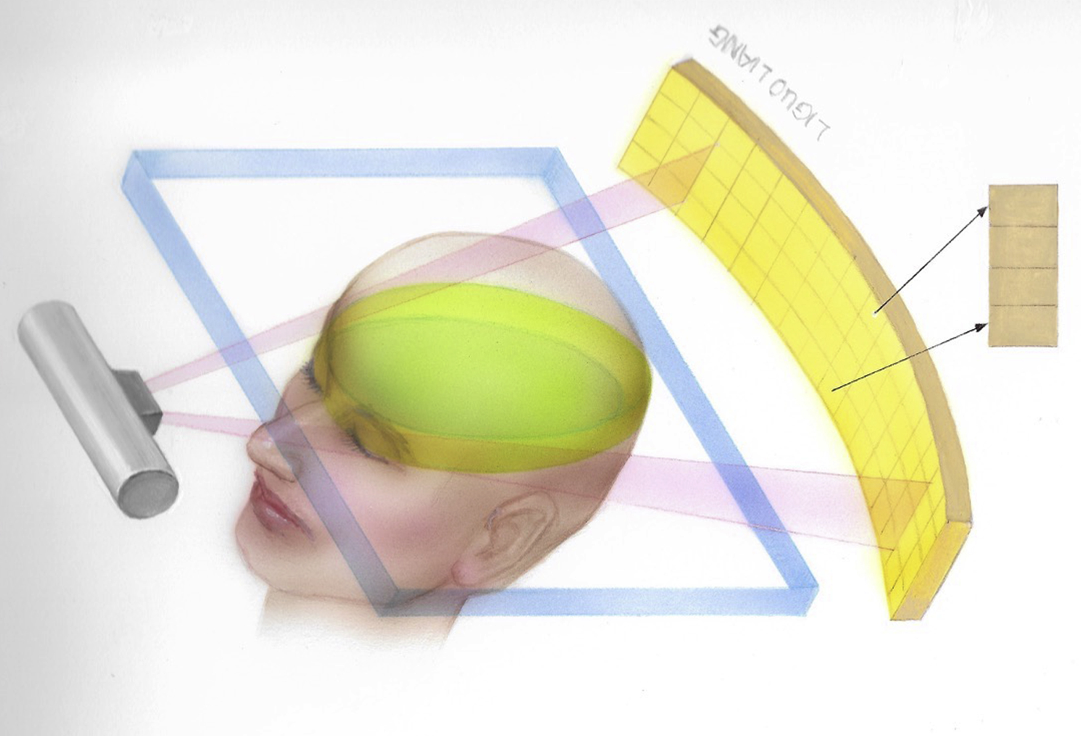
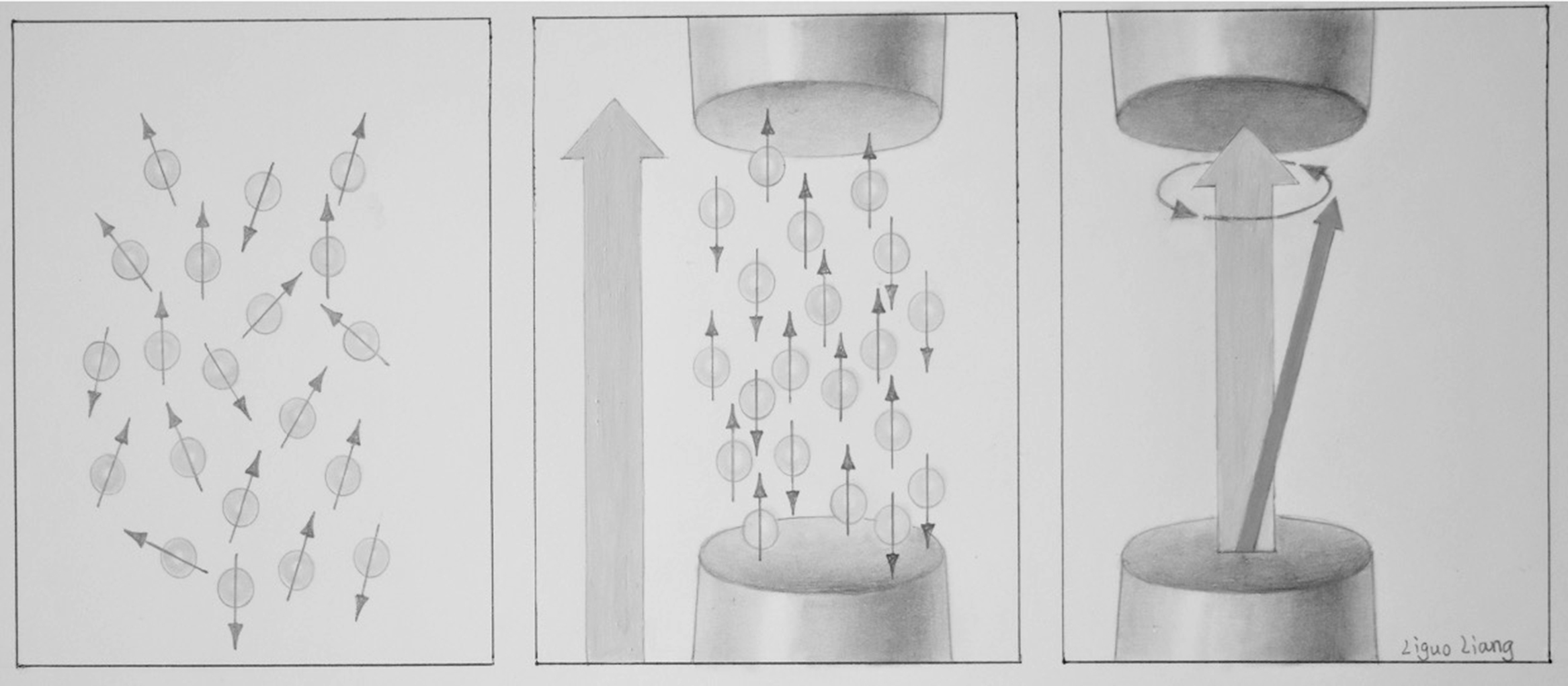
At rest, nuclei precess about B 0 , but since they are all randomly oriented with respect to each other, there is no detectable signal. When external energy in the form of a RF magnetic field is applied at the Larmor frequency, resonance, a natural phenomenon characterized by an oscillating response occurs. The 1 H nuclei are excited out of their equilibrium state into a state of alignment tipped away from the direction of B 0 ; however, they still precess about B 0 , and their precessional motion results in their net nuclear magnetic fields inducing RF currents in nearby conductors, or RF coils, emitting a detectable signal. In the human body, signals vary depending on the tissue type with greater proton density yielding to a higher signal and vice versa. Depending on the surrounding molecules (i.e., tissue type), 1 H nuclei within the magnetic field return to a state of equilibrium at different rates. If the spins aligned with B 0 are added together, they result in a net magnetization vector ( Fig. 2.7 ).
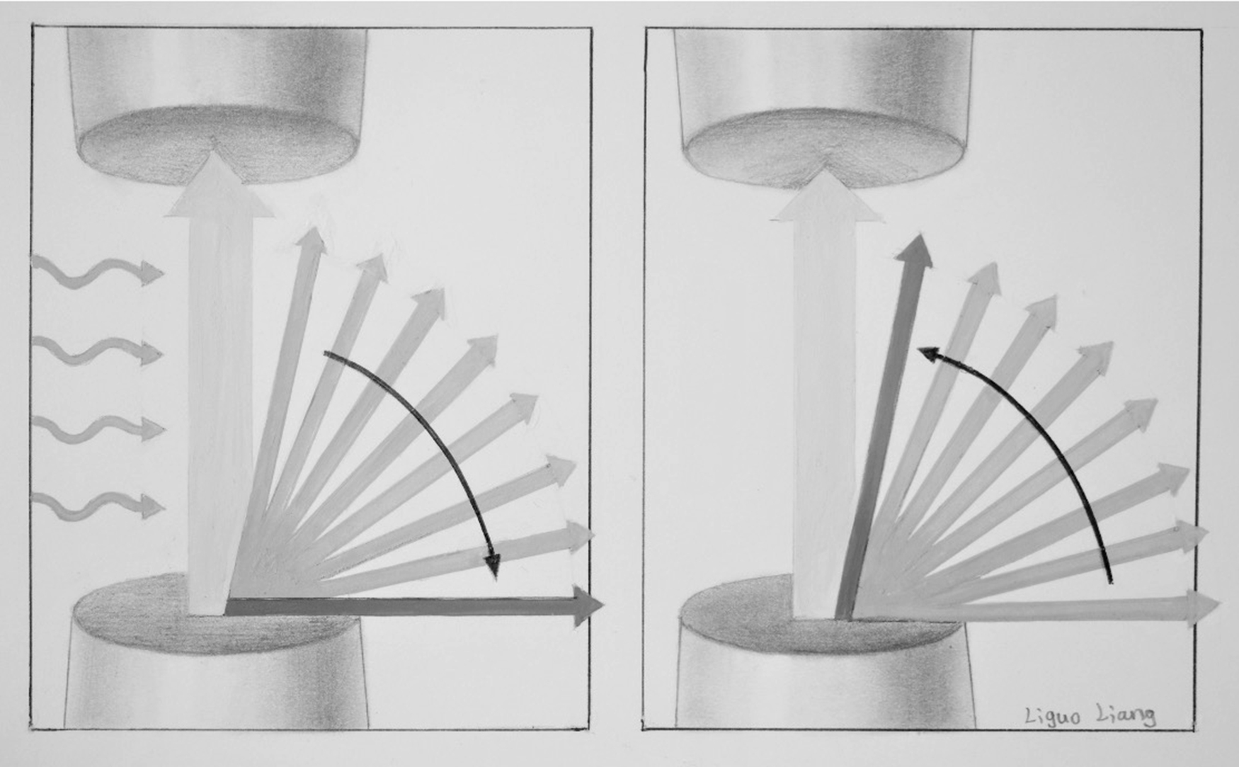
In NMR, free induction decay (FID), first performed by Erwin Hahn, is defined as the observable NMR signal generated by non-equilibrium nuclear spin magnetization precessing around B 0 . In FID, following RF excitation, the magnetization relaxes and the protons undergo dephasing which attenuates the transverse component of the magnetization and causes the signal to decay and energy loss which causes the longitudinal component of the magnetization to recover its equilibrium value. The magnitude of a FID signal is dependent upon a number of parameters such as the sample size and composition, the strength of the magnetic field, and the flip angle (FA). The FA, also known as the tip angle, is the amount of rotation the net magnetization (M) experiences during the application of an RF pulse ( Fig. 2.8 ).
In MRI, after excitation, each tissue returns to its equilibrium state. Longitudinal or spin-lattice relaxation describes the loss of energy from the spins to their environment, causing recovery of the longitudinal component of the equilibrium value M 0 , with time constant T 1. Transverse or spin–spin relaxation is the irreversible dephasing among spins due to microscopic interactions between molecules and nuclei in the transverse direction; it occurs with time constant T 2 . The choice of echo time (TE: the time between the initial excitation pulse and the time at which signal is acquired) and repetition time (TR: the time between successive acquisitions, equivalent to the time between successive excitations) determines the signal contrast. If a short TR is chosen, tissues with long T 1 do not fully recover to equilibrium between successive excitations, thus they produce a weak signal. Alternatively, tissues with short T 1 recover more quickly and produce a relatively strong signal. Table 2.1 shows relaxation times at 3T for some sample tissues. Different pulse sequences may be exploited to produce signal contrast in MRI and these MRI techniques may be adapted to optimize conspicuity of certain structures or pathologies.
Related posts:


Stay updated, free articles. Join our Telegram channel

Full access? Get Clinical Tree


