3 In the process of image formation, a number of scientific attributes and principles come to play that are generalizable across multiple imaging modalities. They are collectively termed imaging science. They include statistical foundations and models associated with image formation and evaluation; principles of error propagation; common metrology of image quality including image contrast, resolution, and noise; and image processing and reconstruction. These topics take special form and consideration in the context of each imaging modality, but they have shared foundations across modalities. Uncertainty and error are inevitable components of the science of medical imaging. The presentation of patient data in the form of images involves uncertainty and statistical variability at multiple levels for all imaging modalities. An appreciation of error allows the interpreter of images to judge the value of visual data and to develop more informed decisions about techniques of image acquisition. Each imaging system is operated by a set of parameters that defines the acquisition condition such as the pulse sequence parameters in magnetic resonance imaging (MRI) or the flux of the radiation and its energy (e.g. kV, mA, and time) in X-ray-based imaging. Trade-offs among these and other variables are dealt with continuously in diagnostic imaging. The choice of these technique factors influences the statistical fluctuations in the image data in the form of noise. Noise is the random variations in displayed pixel value present in all forms of medical images. Acquisition of imaging data is influenced by uncertainties that arise at all stages in the image-forming process. In MRI, the wide variety of choices among variables such as pulse sequences, field strengths, and receiver coils affect the signal strength and its corresponding statistical fluctuations. In X-ray imaging, noise is often dominated by the limited number of photons used to form the image. Given the prevalence of noise, the imaging specialist must obtain a reasonable command of rudimentary statistical concepts. The error of a measurement is the difference between the measured value and the “true value” for the variable being measured. Two categories of error exist: determinate and indeterminate errors. Determinate, also called systematic, errors result from factors such as inadequate experimental design, malfunctioning equipment, and incomplete correction for extraneous influences. The influence of determinate errors on experimental results can often be reduced by better instrumentation and thorough planning and execution of an experiment. For imaging systems, some examples of determinate errors include overexposure or underexposure in radiography, incorrect time gain compensation settings in ultrasonography, and a falloff in surface coil sensitivity in MRI. Indeterminate errors, also called random errors, are errors that can be mitigated by correcting extraneous factors but cannot be eliminated. They are caused by fundamental uncertainties in the variables being measured and in the processes of obtaining and displaying the measurements. Indeterminate errors, being random in nature, produce inherently uncertain outcomes and can only be predicted by applicable rules of probability. In nuclear medicine, for example, the random nature of radioactive decay and the statistical uncertainties in detecting ionizing radiation give rise to significant indeterminate errors. A measurement or imaging process aims to ascertain the truth of an entity. Usually, the “true value” for a measurement cannot be determined (if it could, there would be no need for the measurement). The exact “truth” may not be fully attainable. However, a technique may be available that yields results that are generally accepted as being as close as possible to the true value based on technological possibility (because it is practically not possible to attain perfection) or clinical relevance (because the clinical outcome will be the same even if the reality is not fully ascertained). This technique and the result that it provides are referred to as a “gold standard.” An example of a gold standard is the biopsy results against which interpretations of diagnostic images are often evaluated. Correspondence between measurements and the gold standard are characterized in terms of two key concepts, accuracy and precision, as illustrated in Figure 3.1. Accuracy is the correspondence between a measurement (or the average of a series of measurements) and the gold standard. To increase the accuracy of experimental results, the influence of both indeterminate and determinate errors must be reduced. The contribution of determinate errors to a reduction in the accuracy of a set of measurements is termed the bias of the measurements. Bias in the scientific context is different from its meaning in the social context: prejudice or a state of mind that creates a desire for a particular outcome. Figure 3.1 Precision, bias, and accuracy. Distinct from accuracy, precision is the consistency of the results in the repeated measurements. The precision of a series of measurements describes the range or spread of the individual measurements from the average value of the series. Precision is primarily related to indeterminate error and improves as the influence of indeterminate error is reduced. Precision does not describe the accuracy of a series of measurements. Accuracy is achieved only if the measured values agree with the true value determined by some method other than the measurement technique under consideration. A series of events is said to be random if every event has an equal probability of occurring without correlation between them. “White noise,” an example of random noise, refers to the presence of background signals that are random or uncorrelated in nature. The background signals in an image that constitute white noise are “independent events,” which have the property that each event has no influence on the likelihood or value of a previous or subsequent event, whether spatially or temporally. When describing the results of several measurements, a single value that summarizes the results is useful. For example, consider the data in Table 3.1. A typical approach to the problem is to average the data. However, the term “average value” is nonspecific. Specific reporting quantities are more descriptive. Here, we briefly define singular description or data statistics. Table 3.1 Example data for sample calculation of mean, median, and mode The mean is the result obtained by summing all measured values and dividing by the number of values. The sum of the nine values in Table 3.1 is 39. Therefore, the sample mean is 39/9 = 4.3. When values are placed in the order of magnitude (from smallest to largest, for example), the median is the center value, the so-called 50th percentile of the data. Half of the values are greater than the median, and half are less. The data in Table 3.1, when placed in rank order, have the value 4 as the median. As there is an odd number of values, the median is an actual data value. If there were an even number of values, the median would be the average of the two values on either side of a hypothetical center value. The mode is the value that appears most often in a set of data. When the data in Table 3.1 are placed in the order of frequency of occurrence, one can readily notice that the value 6 occurs most often. Hence, 6 is the mode for this series of measurements. The mean, median, and mode are all quantities describing the average of a dataset, but as they are often different, it is important to specify the type of “average” that may be ascribed to a dataset. For example, suppose that the data in Table 3.1 are the scores obtained by radiologists diagnosing a disorder with a new type of imaging system. In these data, a score of 6 represents perfect agreement with biopsy results, and a score of 0 represents complete disagreement. We may compare the mean scores for other imaging systems against the mean score of 4.3 for the new system. The mode, or most frequently reported score, is the high score of 6. Perhaps, the experimental setup should be examined to see whether the viewing conditions, training, experience, or other factors were more favorable for the four radiologists who scored 6. The 50th percentile score (median) was 4, and the next highest score was the maximum. This suggests that the radiologists can be separated into two groups, one whose performance with the new system is excellent and another whose performance is inferior. This conclusion suggests that any differences between the two groups (e.g. training, experience, visual acuity, and viewing conditions) might explain the difference in performance. The standard deviation for a series of measurements describes the precision or reproducibility of the measurements. From a series of N measurements, the sample standard deviation, σs, can be calculated as where r is the mean value of the sample and xi represents individual measurements. The square of standard deviation, Table 3.2 Example data for computation of mean and standard deviation Indeterminate error implies that the results of a measurement may be different if the measurement is repeated. After many measurements have been recorded, a histogram can be constructed to show the number of observations for each measurement value. If the histogram is plotted as the frequency or fraction of times that each measurement is observed, it is called a probability distribution. A probability distribution gives the probability that each specific value will be measured if the experiment is repeated (Figure 3.2). It expresses the likelihood of each of all possible outcomes of a set of measurements. As such, the sum of all likelihoods or probability (i.e. the area under a probability curve) is unity. Figure 3.2 A histogram showing the frequency of occurrence of a variable quantity. A histogram may be presented as bars, points, or a continuous line. An accurate assessment of the probability of occurrence of each value would require an infinite number of measurements. If the sources of indeterminate error are known; however, a choice can be made among different theoretical probability distributions whose properties are depicted by mathematical analysis. There are two types of distributions that are especially relevant to medical imaging: Poisson and Gaussian. A Poisson distribution is a discrete distribution as it may contain only 0 or positive integers. Radioactive decay as a probabilistic (random) process is a good example of a Poisson distribution [1]. When dealing with a single nucleus, the likelihood of delay is a probability only – one cannot say with certainty when it may occur. However, for a group of nuclei, the probability does describe the number decaying within a certain time lapse. The Poisson probability distribution follows the mathematical form where pn is the probability of obtaining a count n, r is the true average value for the sample, and term n! (i.e. n-factorial) equals (n)(n − 1)(n − 2) ⋯ (2)(1). The probability pn is termed the Poisson probability density. As the true average value (often called the true mean) for a sample cannot be determined by 100% certainty, r is often assumed to equal the mean of the measured data (estimated sample mean). If a series of measurements is distributed according to the Poisson probability distribution, the standard deviation σ is given by Figure 3.3 shows the results of an experiment in which the radioactive count rate (number of counts measured over a given counting time) was measured repeatedly. It is important to recognize that a Poisson distribution applies to discontinuous discrete data. The mean is the arithmetic average of measured values. Figure 3.3 Data for 137Cs source that provided a count rate of about 1000 counts/min. Each measurement consisted of 10 000 counts. The results of 100 measurements were plotted as a function of the number of times that the count rate fell within successive increments of 5 (i.e. between 975 and 980, 980 and 985). Source: Hine 2016 [2]. Reproduced with permission of Elsevier. In the condition when a large number of random values is accumulated for a statistical sample, the Poisson distribution curve of a value approaches a normal, the so-called Gaussian, distribution. Figure 3.4 illustrates the approach of a Poisson probability distribution to a Gaussian distribution. Poisson for 1000 counts is more aligned with normal distribution than does the 100-count example. Figure 3.4 Probability of observing a particular count is plotted for 100 (additive) measurements and (additive) 1000 measurements. Dotted curves illustrate normal probability density functions, and solid curves illustrate Poisson probability density functions. Curves have been normalized to equal heights at the mean. A Gaussian distribution is a bell-shaped symmetrical distribution characterized by two key values: the mean of a set of measurements (r) and the standard deviation (σ) of the measurements. The Gaussian probability density gn is mathematically described as where gn is the probability of observing a count n when the true count (estimated as the average count) is r. As the equation implies, the Gaussian distribution is continuous and symmetrical, with both tails extending to infinity and the standard deviation represented by the distance from the mean value to the inflection point of the distribution curve. Contrary to Poisson distribution, if a series of measurements is distributed according to the Gaussian probability distribution, the arithmetic mean, median, and mode are identical. The standard deviation σ, however, as in the case of Poisson distribution is given by In a normal distribution, 68.3% of all measured values fall within 1σ on either side of the mean, 95.5% within 2σ, and 99.7% within the limits of 3σ. As such, if an experiment yields results that follow a normal distribution, there is a 68.3% likelihood that any particular result will fall within 1σ of the mean, a 95.5% chance that the result will be within 2σ, and a 99.7% chance that the result will be within 3σ of the mean. See Figure 3.5 for a schematic illustration. Figure 3.5 The three Gaussian probability distributions shown above are centered about the mean value r for ±1, ±2, and ±3 standard deviations (a, b, and c, respectively). In imaging physics, there are numerous functional dependencies between variables, each of which has its own inherent variability. Propagation of error is a statistical process by which the overall variability in a quantity is derived from the variability of its constituents. For example, counts measured in a nuclear decay follow a Poisson distribution, and as such, the standard deviation is equal to the square root of the mean. However, a count rate obtained by dividing the number of counts by the counting time does not share the same value for the standard deviation. For a general functional dependency of dependent variable w to independent variables x, y, z, etc., where w = f(x,y,z,…), and where each independent variable has its own standard deviation (e.g. σx), propagation of error follows the general equation of The results of this formalism for few simple arithmetic dependencies are noted in Table 3.3. Table 3.3 Error propagation in simple arithmetic operations The precision of A and B is described by the standard deviations σA and σB. α is a constant. Following this formalism, for the count rate example above, the estimated standard deviation σc of a count rate c obtained by dividing the total number of counts n by the counting time t is derived as where σs is the estimated standard deviation of count n. Hence, the estimated standard deviation of a count rate (average or instantaneous) is determined by first dividing the count rate by the counting time and then taking the square root of the result. Standard deviation defined above is a metric of precision. However, in addition to the standard deviation, a number of other methods can be used to describe the precision of data. Only a brief explanation of these methods is provided here; the reader is referred to standard texts on probability and statistics for a more complete explanation [3–5]. Probable error (PE) may be used in place of the standard deviation to describe the precision of data. The probability that any particular measurement will differ from the true mean by an amount greater than the PE is 0.5. The PE is 0.6745σ for Gaussian and Poisson distributions. Confidence limits may be used to estimate the precision of a number when repeated measurements are not made. For example, if a result is stated as A ± a, where ±a defines the limits of the 95% confidence internal, then it may be said with “95% confidence” that a second measurement of A will fall between A − a and A + a. For a normal distribution, the 95% confidence interval is approximately A ± 2σ. Confidence limits are also referred to as a confidence interval, with the limits serving as the lower and upper bounds of the interval. Values of 1-, 5-, 25-, 50-, 75-, 95-, and 99-percentile are frequently used. The fractional standard deviation (σ/r) may be used in the place of the standard deviation to describe the precision of data. If r represents the mean, then where c is the average count rate measured over a time t. Standard error, more properly characterized as the standard deviation of the mean, σm, yields an estimate of the precision of the mean of a set of measurements. For N individual measurements constituting a mean, The standard deviation of the mean is a measure of the spread of mean values expected when the sets of data (such as the 10 measurements in Table 3.2) are repeated several times. If the experiment was repeated once, there is a 68.3% chance that the mean value of the next dataset would fall within ±1 standard deviation of the mean of the first set. The standard deviation of the mean should not be confused with the standard deviation of a set of data. It is misleading to report the standard deviation of the mean instead of the standard deviation of individual values of a set of data unless it has been made clear that the spread of the mean values is the parameter of interest. It is usually the range of individual measurements that is of interest. Under such circumstances, reporting the standard deviation of the mean simply makes the data look more reproducible than they actually are. A number of statistical tests may be applied to a set of measurements. Among them is assessing the statistical significance of data under varying conditions. Statistical significance tests are generally based on the null hypothesis. The null hypothesis is the assumption that a measured value represents the true value of the quantity and that any deviation between the two is purely statistical and not real. The null hypothesis gives rise to two types of errors: type I error is an error such that the null hypothesis is rejected as false even though it is true, and type II error is an error such that the null hypothesis is accepted as true even though it is false. Other hypotheses can be used, but to understand if the hypothesis is acceptable, a statistical test can be used to determine the probability that a deviation from a true value is equal to or greater than the measured value, i.e. that the difference between the measured and true value is not merely statistical in nature. It is the combination of probability theory and mathematics that is the foundation of statistical analysis. Bayesian theory states that the probability of a data event’s occurrence is equal to the probability of its past occurrences multiplied by the probability of its future occurrences. This analysis assumes that the probability of occurrences does not change, so the knowledge of the characteristics of prior events can be used to predict the future outcome. Mathematics using the central limit theorem, least squares analysis, and other methods have been combined with Bayesian theory to produce current statistical analysis methods. However, to apply any statistical test, some assumptions about the data must be made. If the data meet these assumptions, statistical analysis can be applied using parametric tests; nonparametric tests do not make any assumptions about the data. It should be noted that parametric tests are often applied with nonparametric datasets, and the results can be statistically significant. However, how much the data vary from these assumptions can make the potential error in the result larger and difficult to estimate. Therefore, if a parametric test is used to analyze data that do not meet the required assumptions, the value of the results may not follow the standard outcome limits of the test, e.g. confidence levels. For parametric tests, the assumptions are the following: Common parametric tests include Student’s t-test, chi-square test, analysis of variance, and Pearson or Spearman rank. Common nonparametric tests include variations of chi-square test, Fisher’s exact probability test, Mann–Whitney test, Wilcoxon signed-rank test, Kruskal–Wallis test, and Friedman test. As commonly applied tests in conjunction with medical applications, below we review Student’s t-test and chi-square test. Student’s t-test is a method for testing the significance of the difference between two measurements, or two sets of measurements. The t-value for the difference between two measurements n1 and n2 is where σ1 and σ2 are the standard deviations for the measurements n1 and n2, and the vertical bars enclosing n1 and n2 indicate that the absolute or positive value of the difference. With the computed t-value and Table 3.4, the probability p that the difference in the numbers is simply statistical in nature and is not a real difference between dissimilar samples may be determined. Table 3.4 Cumulative normal frequency distribution Values of p > 0.01 are seldom considered indicative of a significant difference in values between measurements. The chi-square test is used to determine the fit of measured data to a probability density function. From a series of repeated measures, the value of χ2 may be computed as where xi represents each of N individual measurements and r is the sample mean. The formula for computing χ2 from a sample resembles the formula for calculating the sample standard deviation (Eq. (3.1)) such that If the variable we are measuring has a Poisson distribution, then the sample standard deviation σs would be close to the square root of the mean r of the sample. That is, the square of the sample standard deviation (the variance) should equal the sample mean. If that is true, then Eq. (3.11) shows that χ2 is equal to N − 1, or one less than the number of data points. χ2 may be used as a measure of how closely the sample data correspond to a Poisson distribution. From the computed value of χ2, the number of degrees of freedom (N − 1), and data in Table 3.5, a probability p may be determined. Values of p less than 0.05 suggest that the data are distributed over a wider range of values than would be expected for a Poisson distribution. Values of p greater than 0.95 suggest that the data are confined to a smaller range of values than that predicted for a Poisson distribution. Table 3.5 Chi-squared values In medicine, there are many instances in which it is necessary to classify a patient or specimen into one of two (i.e. binary) groups: normal/abnormal, diseased/healthy, exposed/unexposed, etc. This classification is a foundational component of most diagnostic tests. Consider a diagnostic test (e.g. blood test, mammography examination, genetic test, etc.) designed to detect abnormal case among a mixed population of mutually exclusive normal and abnormal cases. The test analyzes a case and declares them either negative (normal) or positive (abnormal). There are four possible outcomes of the test for any given case: The first two outcomes are cases where a case was correctly classified, and the second two cases were incorrectly classified. The outcomes can be summarized in a 2 × 2 contingency table: TP, TN, FP, and FN are the total numbers of cases in each outcome group. The total number of cases, N, is the summation of Nnormal and Nabnormal, the number of normal and abnormal cases, respectively (N = Nnormal + Nabnormal). In Table 3.6, a series of statistical metrics are derived from the above quantities to describing the quality of the diagnostic test. Table 3.6 Statistical quantities of diagnostic tests For an imperfect diagnostic test, which applies to essentially all such tests, there is a trade-off between sensitivity and specificity. That is, detecting as many abnormal cases as possible (i.e. high sensitivity) increases the likelihood of incorrectly classifying many normal cases as abnormal (i.e. low specificity). An example case would be a test that declares all cases positive. Such a test renders perfect identification of all abnormal cases but misses all the normal ones. Conversely, achieving very high specificity likely necessitates accepting poorer sensitivity. An example would be a test that classifies all cases as normal, which implies all abnormal cases are misclassified. Receiver operating characteristic (ROC) analysis provides a mathematical framework with which to judge and compare the effectiveness of different binary diagnostic tests [6]. The ROC curve allows one to formally examine this trade-off and can be used to ascribe overall quality to a binary diagnostic test. Previously, a binary diagnostic test was described as a process that examines an individual case (or specimen) and classifies it as normal or abnormal. However, such binary outcomes are generally drawn from an intermediary process of ascribing a scalar value (continuous or ordinal) related to the confidence or likelihood that the case is abnormal, with a higher value indicates that it is more likely that the case is abnormal. This scalar value is called the test statistic, λ. To make a final binary classification decision, the test statistic is compared to some threshold, τ: if λ < T, the case is classified as normal, otherwise as abnormal. In some tests, the test statistic λ is explicitly calculated. For example, in blood tests, a biological quantity (λ) is extracted and compared to a reference value (T). In other tests, λ is implicit. For example, when a radiologist interprets a mammogram image, λ is not formally computed but rather exists as part of a complex cognitive process in which the radiologist is identifying specific image features and patterns, weighing those against his/her vast prior experience, and internally (even if subconsciously) evaluating his/her degree of confidence that the patient is normal or abnormal. When a given diagnostic test is administered to a large population of individuals or cases, λ values are ascribed to each normal (λN) and abnormal individual (λA). Because of the variability among the population being examined, and because of the random variability inherent in most diagnostic tests (e.g. image noise, instrumentation uncertainty, and inconsistent administration of the diagnostic test), λN and λA can both be treated as random variables having statistical probability distribution functions For a given decision threshold T, the statistics described in the last section can all be computed based on the aforementioned probability distributions (see Figure 3.6). Here, we focus on just the statistics relevant to ROC analysis: Sensitivity is given by the area of the abnormal distribution, Figure 3.6 (a) Illustration of the test statistic distributions for normal (blue) and abnormal (light pink) cases. (b–e) Illustrations of how relevant statistics are calculated by integrating different portions of each distribution according to the decision threshold, T. Consider two diagnostic tests: Test-A and Test-B represented in Figure 3.6. Sensitivity and specificity are both parametric functions of the decision threshold, T. That is, changing T yields different paired values of sensitivity and specificity. For example, at a given T for each test, Test-A has a sensitivity of 75% and a specificity of 65%, whereas Test-B has a sensitivity of 65% and a specificity of 75%. Adjusting T yields new sensitivity and specificity values. What values of T should be used to compare the two tests? An ROC curve will alleviate this problem, allow one to compare the two tests over all possible decision thresholds, making the comparison independent of any specific threshold level. An ROC curve is a plot of the parametric curve of sensitivity vs. FPR for all possible values of T. In other words, it is a plot of true positives vs. false positives for varying T. The construction of an ROC curve is illustrated in Figure 3.7. In essence, you slide T from the lowest possible value to the highest possible value in small steps, compute sensitivity and FPR for each step, and plot each resulting point with sensitivity on the y-axis and FPR (i.e. 1 − specificity) on the x-axis. Figure 3.7 Illustration of how an ROC curve is constructed. Given the (a) distributions of λ for both normal and abnormal individuals, a series of decision thresholds are defined, and for each threshold, sensitivity and FPR are computed and (b) plotted against each other to form the ROC curve. Because both sensitivity and FPR are lower-bounded by 0 and upper-bounded by 1, an ROC curve is bounded within these limits on both the x– and y-axes. A perfect diagnostic test would have an ROC curve along the left and upper edges of this bounding box. A useless test would have a diagonal ROC curve, corresponding to a test that randomly flips a coin to classify a case as normal or abnormal. Generally speaking, the more an ROC curve moves toward the upper left corner, the better the diagnostic test (see Figure 3.8). An ROC curve in the bottom right quadrant is making a decision directly opposed to the truth. In those cases, simply flipping each decision from the output of the test (i.e. normal becomes abnormal and vice versa) will reflect the ROC curve about the diagonal. Figure 3.8 Illustration of how different diagnostic tests would have different distributions of their test statistic (a) and subsequently different ROC curves (b). Take note that when the two distributions (normal – blue and abnormal – light pink) have little overlap, the ROC curve hugs the top left corner (see Test-1 for example), indicating an accurate diagnostic test. On the other hand, when there is no separation between the distributions (see Test-4 for example), the ROC curve lies along the diagonal, indicating the poorest possible test. The most common figure of merit used to quantitatively summarize and compare two (or more) ROC curves is the area under the curve (AUC) (i.e. the integral of the ROC). As mentioned above, ROC curves hugging the left and upper edges of the bounding box correspond to diagnostic tests that are highly sensitive and specific over a wide range of decision thresholds. As a curve moves closer and closer to the ideal ROC curve, the AUC increases. AUC has a lower bound of 0.5 (corresponding to a diagonal ROC, also referred to as the “guessing line”) and an upper bound of 1. The AUC value itself has several equivalent interpretations: The most common use of AUC is to compare two diagnostic tests and determine which one is superior. Note that when comparing ROC curves that are based on real-world data, one must use the proper statistical tests to confirm that any differences seen are significant. This will be briefly discussed in the next section. Also note that in using AUC as a figure of merit for comparing ROC curves, one is implicitly assuming that both types of misclassification errors (false positives and false negatives) are equally undesirable. ROC analysis is powerful because it allows one to objectively compare diagnostic tests that may use completely different means to make their diagnoses. It is also independent of a specific decision threshold or clinical “operating point” (i.e. a point on the ROC curve). For example, the task of detecting prostate cancer could be done with a blood test (e.g. prostate-specific antigen screening), a physical examination, biopsy, or imaging. For each of these tests, it would be possible to collect data of patients with and without prostate cancer, construct ROC curves for each test, compute AUC values, and compare their effectiveness. Their effectiveness can be weighed against their costs (including financial, physical, and emotional) to determine the optimal strategy for managing patients at risk of prostate cancer. In practice, ROC curves based on real-world data are never as smooth and clean as those shown here, as analyses are often performed with limited cases and noisy data. There are two primary methods to construct ROC curves from real data: parametric and nonparametric methods. Parametric methods rely on fitting the noisy data to a smooth ROC curve based on assumptions about the distributions of the test statistic. The most common assumption made is that the test statistic is a Gaussian distribution for both normal and abnormal cases (or at least can be transformed monotonically to be Gaussian) [7,8]. Under this assumption, the ROC curve is parameterized by just a few parameters, and thus, the construction of the entire ROC curve is reduced to estimating those parameters given the data. Nonparametric methods do not make any assumptions about the underlying distributions of the data and simply construct the ROC curves empirically and directly from the data. ROC curves constructed in this way are generally less smooth and have fewer “control points” than parametric ROC curves. The number of points along the ROC curve is dictated by the number of unique values of the test statistic λ. A large number of software packages exist that will construct nonparametric ROC curves, and the steps required to code such an algorithm are not complicated and could be quickly implemented into any scientific computing platform. Methods also exist to smooth nonparametric ROC curves based on smoothing the underlying histograms [9]. In order to say that two ROC curves are truly different, one needs to perform a statistical test, with the null hypothesis being that there is no difference in the curves. Most commonly, the AUC of two curves is used as the basis of comparison. The nature of the study used to generate the data (paired or independent groups, ordinal or continuous test statistics, and parametric vs. nonparametric ROC) will determine the specifics of the statistical test. The reader is directed to the references for specific tests used under different scenarios [10–13]. Commonly, however, statistical packages will output confidence intervals of AUC values or confidence intervals of the difference in AUC values. These can be used for making comparative statements about two diagnostic tests. Care should be exercised to properly account for correlations between cohorts (e.g. paired study) when doing the analysis. The image formation process is highly influenced by statistics of energy interaction with the body and with the detector. Several decades of particle physics experiments have thoroughly studied and documented the underlying mathematical and statistical processes that govern energy interactions. In X-ray imaging, which dominates most of medical imaging practice today, for a range of photon energies and atomic numbers, the relative probability of photoelectric and Compton effects are meticulously measured and tabulated. Given this knowledge base, it is possible to fairly accurately model the image formation process using ionizing radiation accounting for the attributes of tissues and detectors, the principles of interaction of radiation and matter (e.g. tissue, filters, and detectors), and underlying probability of interactions. Modeling of imaging process plays a vital part in medical imaging. This is due to the fact that medical imaging science and engineering, compared to other sciences, does not readily lend itself to experimentation; it is unethical to test a system with questionable quality and safety on humans. In cases when clinical trials are possible, often the absolute truth of the patient cannot be known either. Simulation alleviates both of these challenges. As such, imaging simulations have a wide range of applications ranging from design and optimization of imaging systems to patient dosimetry to effectively mitigate the undesirable effects of excessive patient exposure. There are primarily two methods to simulate X-ray and γ-ray imaging processes through the modeling of radiation interactions: Statistical modeling is recognized as the most accurate metrology for imaging simulation. An imaging system can be thought of as a series of radiation interactions where each interaction has an associated uncertainty. These uncertainties and their probability of occurrence are well understood through experimental measurements. Modeling these interactions with their probabilities of occurrence repeatedly can approximate the expected outcome from a medical imaging process. This method of simulating and modeling of a medical imaging system is accomplished using a method known as Monte Carlo, using a name that highlights the statistical (e.g. gambling) nature of the process. Monte Carlo simulation is a mathematical computerized technique that allows for the inclusion of statistical uncertainties and variabilities in the modeling of the outcome of a measurement, in our case medical imaging. The uncertainties associated with radiation interactions are related to statistical models for which a priori knowledge is available. As an example, consider an imaging system has an input radiation beam with energies
Imaging Science
3.1 Introduction
3.2 Basic Statistics
3.2.1 Nature of Error

3.2.2 Singular Metrics of Statistics
xi as measured
Mean
xi rank-ordered
Median
Given value
Value frequency
Mode
6
2
3
1
4
2
2
2
6
3
4
2
6
4
6
4
3
4.3
4
4
6
2
6
6
6
4
6
2
6
 , is known as the variance of the measurements. In the example dataset of Table 3.2, the mean may be expressed as 43 950 ± 380, where 380 is understood to be σ:

xi as measured
Deviation (xi − r)
Deviation squared (xi − r)2
43 440
−510
260 100
43 720
−230
52 900
44 130
180
32 400
43 760
−190
36 100
44 390
440
193 600
43 810
−140
19 600
44 740
790
624 100
43 750
−200
40 000
44 010
60
3 600
43 750
−200
40 000


3.2.3 Probability Distributions

3.2.3.1 Poisson Distribution


3.2.3.2 Gaussian Distribution


3.2.4 Propagation of Error

Operation
Standard deviation of C
C = A + B

C = A − B

C = AB

C = A/B

C = α A
|α| σA

3.2.5 Quantities of Precision
3.2.5.1 Fractional Standard Deviation
 , and the fractional standard deviation (σ/r) is
  . For example, σ for the number 10 000 is 100, and the fractional standard deviation is 100/10 000 = 0.01. The percent standard deviation (%σ) is the fractional standard deviation multiplied by 100. In the example above, %σ = 1. The percent standard deviation of a count rate (%σc) is

3.2.5.2 Standard Error
 , where σs is the standard deviation of the individual measurements. Thus, two factors influence the value of σm: the variability of the original set of measurements, as represented by σs, and the size of the sample N.
3.2.6 Statistical Analysis
3.2.6.1 Student’s t-Test

t-Value
p
t-Value
p
0.0
1.000
2.5
0.012 4
0.1
0.920
2.6
0.009 3
0.2
0.841
2.7
0.006 9
0.3
0.764
2.8
0.005 1
0.4
0.689
2.9
0.003 7
0.5
0.617
3.0
0.002 70
0.6
0.548
3.1
0.001 94
0.7
0.483
3.2
0.001 36
0.8
0.423
3.3
0.000 96
0.9
0.368
3.4
0.000 68
1.0
0.317
3.5
0.000 46
1.1
0.272
3.6
0.000 32
1.2
0.230
3.7
0.000 22
1.3
0.194
3.8
0.000 14
1.4
0.162
3.9
0.000 10
1.5
0.134
4.0
0.000 063 4
1.6
0.110
4.1
0.000 041 4
1.7
0.090
4.2
0.000 026 6
1.8
0.072
4.3
0.000 017 0
1.9
0.060
4.4
0.000 010 8
2.0
0.046
4.5
0.000 006 8
2.1
0.036
4.6
0.000 004 2
2.2
0.028
4.7
0.000 002 6
2.3
0.022
4.8
0.000 001 6
2.4
0.016
4.9
0.000 001 0
3.2.6.2 Chi-Square (χ2) Test

There is a probability of
2
3
4
5
6
7
8
9
10
11
12
3.2.7 Binary Classification
Truth
Normal
Abnormal
Test
Normal
TN
FN
Abnormal
FP
TP
Quantity
Definition
Equation
Accuracy
Fraction of cases correctly classified
(TP + TN)/N
Sensitivity or true-positive rate (TPR)
Fraction of abnormal cases classified as abnormal
TP/Nabnormal
False-negative rate (FNR)
Fraction of abnormal cases incorrectly classified as normal
FP/Nabnormal = 1 − sensitivity
Specificity or true-negative rate (TNR)
Fraction of normal cases classified as normal
TN/Nnormal
False-positive rate (FPR)
Fraction of normal cases incorrectly classified as abnormal
FP/Nnormal = 1 − specificity
Positive predictive value (PPV)
Fraction of cases classified as abnormal who were actually abnormal
TP/(TP + FP)
Negative predictive value (NPV)
Fraction of cases classified as normal who were actually normal
TN/(TN + FN)
3.2.8 ROC Methodology
3.2.8.1 Test Statistic
 and
and  , respectively. The corresponding cumulative distribution functions are denoted as
  and
and  , respectively.
3.2.8.2 ROC Curve
 , integrated after the decision threshold (Figure 3.6c), thus sensitivity =
  . False-negative rate (FNR) is given by the area of the abnormal distribution,
  , integrated before the decision threshold (Figure 3.6e), thus FNR =
  = 1 − sensitivity. Specificity is given by the area of the normal distribution,
  , integrated before the decision threshold (Figure 3.6b), thus specificity =
  . In addition, false-positive rate (FPR) is given by the area of the normal distribution,
  , integrated after the decision threshold (Figure 3.6d), thus FPR =
  1 − specificity.

3.2.8.3 Anatomy of an ROC Curve

3.2.8.4 Area Under the Curve, AUC
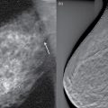
3.2.8.5 Practical Applications of ROC Analysis
3.3 Modeling Radiation Interactions
3.3.1 Monte Carlo Simulations

Related posts:
![]()
Stay updated, free articles. Join our Telegram channel


Full access? Get Clinical Tree


