10 Medical imaging, as practiced today, exploits the unique attributes of the human tissue, for example, its X-ray absorption, radiopharmaceutical distribution, and ultrasonic interaction to extract relevant information for medical purposes. Among these attributes are the body’s magnetic properties. Although these properties are subtle in everyday environments when the body is positioned in a strong magnetic field, they become large enough so that they can generate a high-enough signal to extract useful information in the form of images. The signal is highly dependent on the way the magnetic field is manipulated, making it possible to obtain multiple image contrasts that are highly diverse and revealing toward different medical needs. This makes the field of magnetic resonance imaging (MRI) highly specialized such that its effective use requires a deep understanding of its unique physics. In this chapter, we first cover the fundamentals of magnetic resonance and then apply this knowledge through different types of MR data acquisition techniques to produce varying image contrasts for tissue as well as analysis of different physiological features and chemical properties of the body. Certain nuclei have net magnetic properties as discussed in Chapter 1. By the use of magnetic fields and radio-frequency (RF) waves, these properties can be exploited to yield information about the biological materials containing such nuclei. There are two different perspectives used to explain the phenomenon of magnetic resonance, classical and quantum mechanical. The classical perspective is more intuitive and useful for understanding most aspects of MRI. The quantum mechanical perspective offers a more accurate microscopic behavior of nuclei in an external magnetic field. The two interpretations merge (as they must) when describing the macroscopic phenomena, i.e. the expectation value of quantities of interest describing large populations of nuclei. The energy of interaction of a single nucleus that possesses a magnetic moment with an external magnetic field is given by where the magnetic moment of the nucleus where e is the charge of the proton in coulombs, ℏ is the Planck’s constant divided by 2π, Mp is the mass of the proton, and μB is the Bohr magneton [1]. In the quantum mechanical derivation, this is modified to where the so-called g factor corrects the value of the classical magnetic moment and I has been rewritten as the spin angular momentum quantum number for the proton multiplied by ℏ. Combining the fundamental constants in Eq. (10.3), this is rewritten as where γ is called the gyromagnetic ratio. Assigning the z-axis in the coordinate system to be along B0, Eq. (10.1) is reduced to the projection of Combining Eq. (10.4) with Eq. (10.1) for a spin ½ proton, we can obtain This equation describes two energy levels for a proton, which are directly proportional to the strength of the external magnetic field, shown as a plot of energy vs. magnetic field in Figure 10.1. Figure 10.1 Energy level diagram for a spin ½ system. Energy is directly proportional to the external field, B. At a particular B = B0, the difference between the upper (excited) state and lower (ground) state can be equated to a photon of energy ħω0. The conventional way to extend this to an ensemble of protons is not to formally add the interaction terms to the expression for the energy but to assume that (i) B0 polarizes the sample so that the entire population has only one of two possible orientations (μz = ±½ℏ) and that (ii) the difference in the number of protons in the higher excited, Nes, state and the lower ground, Ngs, state is governed by a Boltzmann distribution, which is a function of the temperature, T, of the sample and the size of B0: where Ees and Egs are the energy for the excited and ground states, respectively, and k is the Boltzmann constant. There exists a dynamic balance between the two basic energy states determined by magnetic field and temperature. Nuclei are said to be in “thermal equilibrium” when the number of transitions from the lower to the upper state is equal to that from the upper to the lower state (see Figure 10.2). At biological temperatures for the clinical range of B0, there is only a slight excess of protons in the ground state. For instance, for a magnetic field equal to 1 T, the excess number of protons in the ground state expressed as a fraction of the total number of protons is only about 3 × 10⁻⁶. This is at once both a disadvantage and an advantage of MRI compared to X-ray techniques. It is a disadvantage because the small fraction of protons in the ground state leads to a very weak signal, but it is an advantage because this fraction can change significantly by differences in thermal fluctuations in different tissue environments. This change is the primary source of the soft tissue contrast of MRI compared to X-ray images. Figure 10.2 At equilibrium, there is a slight excess of spin population, Ngs > Nes. Transitions are induced by irradiating with a photon energy that corresponds to the difference between states Egs and Ees. The absorption of a photon with energy equal to the difference between the two states can promote protons from the lower to the higher energy state. The term “flip” is often used because the end result is the change of the proton orientation where the z component has “flipped” from parallel to antiparallel. The expression for the energy of the photon also gives its frequency, ω0, as For clinical magnetic fields, ω0 is in the radio frequency part of the electromagnetic spectrum, orders of magnitude smaller than X-ray energies, and not sufficient to cause ionization. It is no accident that, although derived from quantum mechanical considerations, Eq. (10.7) is identical to the results derived from classical principles. The above extension from the two-state solution for a single proton to an ensemble is actually incorrect in several respects. If done correctly, using interaction terms characterizing thermal effects, the more rigorous quantum mechanical formalism provides a more accurate interpretation. Yet, the majority of MRI can be described using a classical interpretation, and the differences between the quantum mechanical solution relative to the classical model will be described when appropriate in this text. The result of the preceding section is that the magnetic resonance phenomenon can be viewed simply as the energy absorption of a photon between a ground state and an excited state whose energy levels are split by an interaction between an external magnetic field and an intrinsic magnetic moment of a particle, in this case a proton. Although at biological temperatures the population difference between these two states is only a few per million, the number of protons in tissues is more than enough to provide a measurable signal. For instance, the number of protons in a milliliter of water is 6.68 × 10¹⁹. When measuring the aggregate behavior of such large numbers of protons, the classical laws of electromagnetism can be used to explain many features of magnetic resonance. In the classical interpretation, the behavior of a single proton with respect to its position and movements are assumed to be continuous and predictable. At a microscopic level, the quantum mechanical interpretation is that these cannot be specified with any desired degree of precision. The conflict between classical and the quantum mechanical model can be resolved by considering the subsets of the entire population of protons that behave identically in the magnetic resonance process. For example, suppose the external magnetic field was not uniform across the entire tissue sample. Protons in different physical locations would experience different magnetic fields and thus absorb energy (i.e. photons) of different frequencies. The variations in clinical magnetic fields are typically on the order of a few parts per million. However, with ∼1016 protons/ml of tissue available, there are huge numbers of protons (i.e. a subset of protons) at each different magnetic field. Thus, the aggregate behavior of each subset should follow the same course as a single proton, at least in this case of energy absorption, and each subset is large enough so that classical physics should apply. This subset population is sometimes referred to as an isochromat, i.e. same color, in analogy to atomic absorption physics where the same color refers to the same energy transition. Therefore, in the following discussions, the concept of a single proton will be interpreted as an isochromat, although for simplicity and consistency with the literature, “proton” or “spin” will sometimes be used interchangeably. In the classical interpretation, the observation that a proton has a magnetic moment can be explained by assuming that a proton is a uniform spherical distribution of charge, spinning about an internal axis of rotation. Using the laws of electromagnetism, this time-dependent charge distribution produces a vector magnetic field equal to that of a magnetic dipole (see Figure 10.3). Figure 10.3 Magnetic moment of a proton. (a) The basic unit of magnetism is the magnetic dipole whose lines of force are depicted as traveling from the north to the south pole of a bar magnet. The magnetic moment is a vector quantity represented by the green arrow. (b) The proton can be viewed classically as a solid sphere of charge spinning about an internal axis, which results in a magnetic dipole moment whose lines of force are analogous to the bar magnet. Whenever there are multiple sources of magnetic fields present, i.e. magnetic moments, there will be a force of interaction between them, the north pole of one magnetic moment attracted to the south pole of another. In a typical sample of proton-containing material (e.g. the human body), the force of interaction between the individual proton magnetic moments is weak and cannot overcome the effects of other processes, notably thermal fluctuations, and at thermal equilibrium, the proton magnetic moments are oriented in random directions. If a strong external magnetic field is applied to the sample, the energy of interaction, governed by Eq. (10.1), is minimum when an individual magnetic moment is parallel to the external field and maximum when it is antiparallel. In the absence of other considerations, the minimum energy configuration of this system is when the protons “align” their magnetic moments with the direction of the magnetic field in a manner similar to a compass needle aligned with the earth’s magnetic field. It must be stressed that in a real tissue sample, there are other competing forces, and at any given moment, an individual proton magnetic moment may be oriented in any direction, but the average over the whole ensemble results in a small excess in the direction of the external magnetic field analogous to the thermodynamic discussion governed by Eq. (10.6). As the proton has intrinsic angular momentum, the force of interaction between the proton magnetic moment and the external magnetic field produces a torque that is equal to the time rate of change of the proton’s intrinsic angular momentum, I, as From Eqs. (10.3) and (10.4), Equation (10.9) describes a physical picture in which the time rate of change of the magnetic moment position is perpendicular to its position at any time t. The solution to this equation is a precessional motion about Figure 10.4 Classically magnetic dipoles precess with angular momentum ω about the direction of a static field B0 (shown in a) in a manner that is analogous to the precession of a gyroscope as it spins around its own axis under the force of the earth’s gravitational field (shown in b). In both cases, this produces a torque τ, which is perpendicular to the internal axis of rotation. If you push against a stationary ball with no angular momentum, it will roll in the direction in which it was pushed. If you push against a gyroscope, the gyroscope will move in a perpendicular direction (i.e. 90°) to the direction of the push. If you push on the gyroscope in the same direction as the earth’s gravitational field, the gyroscope will precess faster. If you pull the top of the gyroscope vertically, i.e. opposite the direction of the force of gravity, the gyroscope will precess more slowly. In the macroscopic world, rotating objects that have angular momentum behave as gyroscopes and tops. In the classical interpretation of magnetic moments, the observation that nuclei react to forces just as objects in the macroscopic world was explained by assuming that protons and other subatomic particles rotate about their internal axes and are described as having “spin.” In the absence of any other forces, the solution to Eq. (10.9) is a precessional motion with angular frequency termed the Larmor frequency, named after the English physicist Sir Joseph Larmor who derived the equation in order to explain the splitting of atomic absorption spectra in the presence of a magnetic field [1]: The frequency of precession of a proton in units of megahertz (106 cycles/s) is given by f = ω/2π and depends on its gyromagnetic ratio γ (usually written in megahertz/tesla) and the strength B (in tesla) of the static magnetic field. Gyromagnetic ratios for a number of nuclei are given in Table 10.1. Table 10.1 Magnetic resonance properties of selected nuclei aThe gyromagnetic ratio listed here is the same value listed in some texts as γ/2π, where γ is the gyromagnetic ratio in units of radians/tesla. The convention in this text is to assume that γ is given in the units of megahertz/tesla, with the factor of 2π already included. bRelative sensitivity (i.e. signal strength as compared with hydrogen) for the same number of nuclei at constant field strength as a percentage of sensitivity for 1H. Source: Data from James [2] with permission of Elsevier. Equation (10.10) assumes that the only magnetic field the protons see is the external laboratory field; however, magnetic fields associated with the nearby electrons will add or subtract from the external field at the proton depending on their molecular distribution. Because of this, Eq. (10.10) is rewritten as where B0 is the explicit designation for the external laboratory field and σ is called the chemical shift or chemical shielding constant. This is a first-order approximation. The deviation in the magnetic field is better described with σ characterized by a tensor quantity. This frequency shift can be measured and used to characterize protons in different molecular environments. This is relevant to the discussion of magnetic resonance spectroscopy (MRS) (see Section 10.8). For routine clinical MRI, the only tissues with large enough number of protons to produce a measurable signal intensity are water and fat. Unless noted specifically, the imaging discussion will assume a single-proton source (i.e. water) and use Eq. (10.10) instead of Eq. (10.11). If we consider the aggregate behavior of a large population of protons, we can first perform a vector addition of all the proton magnet moments in the sample. Such a vector sum is called the bulk magnetization of the sample and has a vector magnetic moment Figure 10.5 Representation of bulk magnetization The distribution of the proton magnetic moments will change because of thermal fluctuations that compete with the magnetic interaction between Figure 10.6 Three-dimensional (3D) representation of proton magnetic moments. (a) In the absence of an external magnetic field, random thermal fluctuations produce a spherical distribution of magnetic moment orientations. (b) The presence of an external magnetic field produces a slightly higher density of orientations in the direction of Figure 10.6 presents a decidedly different picture than Eq. (10.6) and Figure 10.2. Equation (10.6) implies that the effect of B0 is to polarize the sample such that every proton has only two possible projections, i.e. μz = ±½ℏ, and that the only difference is the amount of protons with projections parallel and antiparallel. Consider the picture using isochromats rather than individual protons. As the isochromat is a classical entity, there is no restriction on its orientation, and as the thermal fluctuations are random, the distribution of isochromats should be random, altered only slightly by the presence of B0. It turns out that in the limit of high temperatures and at clinical B0 values, the two-state solution extended by the Boltzmann distribution and the more rigorous quantum mechanical statistical treatment converge to the same answer (i.e. Eq. (10.6)). A more detailed discussion of this can be found in a paper by Lars Hanson [3]. In practice, the difference in these two descriptions does not impact the general discussion of MRI with one notable exception, that is, in the effect of applying an RF pulse. The coordinate system used to describe the precessional motion of proton magnetic moments has its z-axis parallel to Figure 10.7 Coordinate system for the vector model of magnetic resonance. (a) The coordinate system has its z-axis parallel to A time-varying magnetic field will induce a current in a nearby conductor according to Faraday’s law of induction. If Btotal is static, M is also static. Therefore, in order to induce a measurable signal in a nearby conductor, a second external magnetic field is introduced, which is time varying. When an additional force is applied to an object with angular momentum in the direction of precession for a period of time and then removed, the resultant precessional frequency will remain unchanged, but the angle with respect to the internal axis of rotation and the direction of the external force will have changed. The best way to visualize this is to consider the motion in a coordinate system rotating at the Larmor frequency ω (see Eq. (10.10)): In such a rotating frame of reference, the precessing proton would appear stationary. If a second magnetic field where Δt is the time B1 is “on.” This time-limited magnetic field is commonly referred to as an “RF pulse.” The angle α is sometimes called the “tip” angle because the net effect is to tip Figure 10.8 Bulk magnetization is rotated away from the z-axis if a radio-frequency field is applied of amplitude B1 rotating synchronously (i.e. in resonance) with the protons. The angle α is proportional to the duration of the RF pulse. A The motion of magnetic moments during the application of an RF pulse in the laboratory frame is the sum of a precession about Figure 10.9 Effect of a 90° pulse. (a) The effect of a In general, for most MRI applications, motion during the RF pulse interval is ignored. Before the RF pulse, the precessing x and y components cancelled out and the vector sum Figure 10.10 Free induction decay (a) after a 90° pulse the magnetization is wholly in the transverse plane (Mt) and precesses about B0 at the Larmor frequency. The amplitude in the xy-plane decreases with time and the magnetization vector traces out a spiral. (b) A magnetic field with time dependence such as this will induce a sinusoidal voltage in a nearby conductor that will be reduced with time as the amplitude decreases. When an RF pulse is applied to a sample, a portion of the bulk magnetization will be rotated into the xy-plane and induce a voltage in a nearby conductor. This signal decays away in the period after the RF pulse is switched off. This decay is the result of the return of protons to the state that existed before the RF pulse was applied. This process of the bulk magnetization returning to its original alignment with the static magnetic field is termed relaxation. Immediately after a 90° pulse, Mz is zero and Mt is at its maximum value. During the FID period, Mz gradually increases approaching the original value of M0 and Mt decreases approaching zero. These two processes are independent. The first process is called longitudinal or spin–lattice relaxation and is characterized by a time constant T1. The term spin–lattice refers to the interaction of the protons with their surroundings (i.e. the “lattice” or network of other magnetic moments). The second process is called transverse or spin–spin relaxation and is characterized by a time constant T2. Spin–lattice and spin–spin are terms originating from the quantum mechanical treatment. In one of the original papers describing magnetic resonance, Bloch formulated a phenomenological approach for these processes [4]: where Consider the period before any RF pulses are applied. In the absence of a magnetic field (i.e. B0 = 0), thermal processes result in an average A plot of this equation for a T1 = 750 ms is shown in Figure 10.11. This curve represents the growth of the longitudinal magnetization after tissue has been placed in an external magnetic field oriented in the z direction. Figure 10.11 Recovery of longitudinal magnetization. The growth of the component of the magnetization M along a magnetic field B0 oriented along the z-direction following a 90° pulse. At t = T1 (i.e. 750 ms in this example), Mz has reached a value After a 90° pulse is applied, where M(tRF) represents the value of a component of M in the transverse plane immediately after the RF pulse. Note that in the free precession period, the Bloch equations are uncoupled, so the solution for the z component is the same as Eq. (10.15). An example of the change of the transverse magnetization (Mt) following a 90° pulse is shown in (Figure 10.12). The time dependence of Mt during the free precession period is an exponential decay. Figure 10.12 Decay of transverse magnetization in the rotating frame following a 90° pulse. At t = T2, i.e. 100 ms in this example, Mt has reached a value of 1/e or approximately 37% of M90, the value of Mt immediately after the 90° pulse. At t = 5xT2, Mt has decayed to less than 1% of M90. These equations and figures depict the behavior of In the classical view, the mechanism for return to equilibrium expressed by Eq. (10.14) requires magnetic fields in addition to B0 and B1, which cause rotations of the proton magnetic moments either toward or away from the z-axis. These additional magnetic fields originate from molecular electrons whose magnetic moments are ∼2000 times larger than the proton magnetic moment. These interactions are most efficient at causing a rotation when these extra magnetic fields have a time dependence analogous to B1, i.e. the magnetic fields are rotating near the Larmor frequency. The sources of additional magnetic fields are the rotations, translations, and vibrations of the molecules on which the electrons reside. The mechanism for the exponential decay of Mt expressed in Eq. (10.15) also involves additional magnetic fields from molecular elections with one notable addition. Immediately after the 90° pulse, individual magnetic moments have been rotated such that the vector sum is in the transverse plane, but each individual isochromat is at a specific phase angle with respect to a reference point and a relative phase angle with respect to the other isochromats. In the absence of any additional magnetic fields, these isochromats would precess at the Larmor frequency maintaining their relative phase angles; i.e. the vector sum Mt would precess at the Larmor frequency theoretically without decay. Additional magnetic fields can change the phase angle and/or the frequency of individual isochromats. The time evolution of the phase of individual isochromats can be split into two components: (i) differences in phase because of constant differences in the precessional frequency and (ii) random phase shifts because of fluctuating magnetic fields. Both types contribute to the decay of the signal by a mechanism known as dephasing. Figure 10.10 depicts Mt diminishing as a function of time tracing out a spiral path as it approaches zero. The vector sum is maximum immediately after the 90° pulse when the distribution of the phase angles of the individual isochromats is smallest. At this time, the individual isochromats are said to be in phase or phase coherent. As Mt evolves over time, the distribution of phase angles gets larger as individual isochromats’ phase changes with respect to one another, resulting in a decrease in the magnitude of Mt (see Figure 10.13). The isochromats are now said to be out of phase or having a loss-of-phase coherence. Figure 10.13 Dephasing of transverse magnetization following a 90° pulse. At t = ta, the phase is advanced for an isochromat precessing at a higher frequency (H) relative to one precessing at a lower frequency (L) and Mt has been reduced by about 10%. At t = tb, tc, and td, the relative phase differences increase and the vector sum Mt decreases until the vector sum is zero. The time constant that describes the total loss of phase coherence from all processes is given the label T2* to distinguish it from those processes that are attributed only to tissue-specific properties. T2* contains contributions from inhomogeneity of the static laboratory magnetic field, which can vary as a function of the design and/or construction of a particular magnet. In some circumstances, this can lead to extremely short T2* with almost complete loss of phase coherence within a few microseconds. This has two consequences: (i) a significant loss of signal-to-noise ratio (SNR) and image quality, particularly given the need to extend data acquisition time to accommodate spatial encoding strategies (see Section 10.3.1) and (ii) the possibility that some image contrast mechanisms could be a function of equipment design and vary between institutions instead of being dependent only on tissue properties. Given the multiplicative property of exponential decay, i.e. ea+b = eaeb, we can separate these contributions by using the following definition: where T2′ contains contributions that are static in time and T2 contains time-varying contributions that arise from the properties of tissue, sometimes referred to as the “true” T2. The main contributing factor to T2′ is inhomogeneity in the static field B0, but could also contain contributions from tissue structures. Using the definition in Eq. (10.17) to replace T2 by T2* in Eq. (10.16), we see that the dephasing effects of the “true” T2 and T2′ are multiplicative, allowing for the possibility that dephasing from T2′ processes could be compensated for independently and measurement of the remaining signal a reflection of tissue properties alone. Reversing the dephasing because of T2′ may also be necessary to extend the period over which the measurable signal can be obtained. This can be accomplished in the following manner. In the period after the 90° pulse, Mt decays with time constant T2* as each isochromat accrues a phase angle proportional to the total magnetic field at that location. Protons in stronger magnetic field environments precess at higher frequencies and accumulate larger phase angles relative to protons in weaker magnetic field environments, leading to a loss-of-phase coherence (see Figure 10.13). Now, however, at time τ, a second RF pulse can be introduced whose amplitude and duration are such that the individual isochromats are rotated 180° about an axis so that their phase angle is the negative of what it was right before the pulse (see Figure 10.14). If the magnetic field at each location is the same as before the pulse, i.e. it does not vary in time, each proton will accumulate a phase angle at exactly the same rate in the interval after the 180° pulse as it did between the 90° and 180° pulses. The result is that at a time equal to 2τ, each isochromat has the same phase it did at t = 0 and phase coherence is re-established. The ensemble is said to be rephrased, and this type of 180° pulse is referred to as a rephasing pulse. The FID signal produced by this sequence is shown in Figure 10.15. The amplitude decays with time constant T2* during the first interval and then grows with the same time constant as the isochromats rephase. After 2τ, the isochromats dephase again analogous to the period right after the 90° pulse. The signal at 2τ has the same form mathematically and appears to “echo” the FID produced by the initial 90° pulse; hence, the term spin echo is used to describe this process. The time interval 2τ is referred to as the echo time, with label TE (time to echo). Figure 10.14 Spin echo formation. (a) A 90° pulse is applied along the negative x-axis, rotating Mt to the y-axis. (b) A 180° pulse is applied along the y-axis at time τ after the 90° pulse. Dephasing occurs during the period between the two pulses with protons at larger magnetic fields precessing at higher frequencies (ωH) than protons at smaller magnetic fields (ωL). Immediately after the 180° pulse, proton phase angles are the negative of what they were before the pulse. (c) In the period after the 180° pulse, protons precess through the same relative phase angle as in the period between the 90° and 180° pulses, bringing them exactly back into phase at time 2τ, called the time to echo (TE). Figure 10.15 Spin echo pulse sequence. A pulse sequence diagram showing signal evolution with the application of a 90° pulse followed by a 180° pulse τ seconds later. The initial FID decays with time constant T2*. The 180° pulse inverts the phase of individual isochromats leading to a rephasing of the magnetization with maximum at 2τ (i.e. TE), referred to as a spin echo. Rephasing is incomplete as the 180° pulse does not account for phase shifts from time-varying magnetic fields and the maximum amplitude of each spin echo FID decays with time constant T2. To assist interpreting how and when pulses are applied, pulse sequence diagrams are made. The spin echo pulse sequence diagram and signal evolution are shown in Figure 10.15. Note that the signal at TE “echoes” the initial FID, but the amplitude is reduced. The assumption that the phase accumulation in the period after the 180° pulse is equal to that before the 180° pulse is valid only if each proton precesses at a constant frequency throughout the two time intervals. Randomly fluctuating magnetic fields from nearby molecular electrons add to the total magnetic field at each proton, so the actual phase accumulation is an integral over each interval of infinitesimal changes in the precessional frequency. Therefore, the phase changes over each interval are no longer exactly equal, leading to an incomplete rephasing at TE. However, the dephasing due to constant differences in magnetic field at each proton (i.e. T2′) will be removed, so the decay of the spin echo amplitude reflects the “true” T2, which is a property of tissue and by collecting echoes with different TE, the decay curve can be measured and the T2 value determined. Although this incomplete rephasing leads to a reduced SNR, the use of the spin echo pulse sequence results in a significant expansion of the time interval over which measurable MR signals can be detected. This extra time is necessary for the addition of spatial encoding of the signal (see Section 10.3.1). The properties of a material that give rise to observed values of T1 and T2 are complex. An early theory of the contribution of molecular motion to relaxation was suggested by Bloembergen et al. in 1948 [5]. An important characteristic in this theory is the definition of a correlation time for molecules. Molecules in liquids and semisolids are free to rotate. The rate at which they rotate is the rotational frequency. The inverse of the rotational frequency is the rotational period, also called the correlation time τc. Molecules that rotate more slowly have a greater probability of interacting with their neighbors. In such materials, relaxation can occur more rapidly and the relaxation time constants are smaller. For T2 relaxation, the prediction shows that a longer correlation time implies a faster transverse relaxation (shorter T2) (see Figure 10.16). For T1 however, there is a resonance phenomenon to consider. Molecules rotating at Larmor frequencies maximize their rate of interaction with their neighbors, just as the interaction of radio waves with magnetic moments is maximized at the Larmor frequency. Thus, a material having a correlation time that happens to coincide with the inverse of the Larmor frequency yields the minimum T1. Materials having smaller or larger values of correlation time have a larger T1. Furthermore, because T1 depends on the Larmor frequency, T1 increases as the magnetic field strength is increased, i.e. materials with correlation times near the resonance value for one field strength would have a short T1 at that field strength only. Figure 10.16 Relaxation times T1 and T2 as a function of correlation time, τc. This is the data for static magnetic field strength of 1.4 T, with proton resonance frequency of 60 MHz [6]. T2 is always shorter than T1. That is, isochromats always dephase faster than the return of the bulk magnetization to equilibrium. For typical biological materials, T1 may be on the order of several hundred milliseconds, whereas T2 is a few tens of milliseconds (Table 10.2). Table 10.2 Relaxation times (mean ± standard deviation) for various tissues at 1 T static magnetic field strength (i.e. proton resonance frequency = 42.6 MHz) aAverage of medulla and cortex. Source: Bottomley et al. 1984 [7]. Reproduced with permission of John Wiley & Sons. Any measurement technique that exploits differences in MR characteristics between tissues enhances the contrast in the image, just as contrast in computed tomography (CT) is influenced by factors such as electron density and physical density, contrast in MRI is influenced by differences in relaxation parameters (i.e. T1 and T2) as well as the number of nuclei (i.e. nuclear spin density and number of spins/cubic centimeter) between tissues. T1 and T2 values can be considered physical properties of biological materials. However, there are difficulties in characterizing tissue with unique values either by direct measurement or by an analytical expression. Bloembergen’s model described above is most appropriate for relatively pure substances in solution. This is not the case for complex tissues that are mixtures of many different substances in different environments with physical barriers to the movement of molecules (e.g. macromolecules, cellular organelles, cell membranes, etc.). Another influence on relaxation times is the temperature of the tissue. The rate of interaction between spins and their surroundings is a factor in determining the rate at which the system returns to equilibrium after an RF pulse. Molecules in a sample are in constant motion and rotate with frequencies that range from zero up to a maximum value determined by the temperature. Any magnetic moment is influenced by the rotation of nearby magnetic moments. As a result of these interactions, isochromats may be rotated toward or away from the z-axis, which affects T1, and they may also move out of phase with other isochromats, which affects T2. A number of other interactions also play a role, although a discussion of which is beyond the scope of this text [7]. A model that would predict T1 and T2 of tissue would not only have to incorporate all of these mechanisms but also include compartment analysis in which molecules exchange energy via magnetic interactions or exchange protons chemically or physically between environments, each with potentially different rate constants. For example, water is known to hydrogen bond to proteins and other macromolecules, resulting in multiple layers with correlation times associated with the larger molecule. This is substantially different than a water molecule freely rotating in solution (e.g. cytosol). There are also differences between intracellular and extracellular water and the rate of exchange between these compartments. Although all these factors make it difficult to construct an analytical model that accurately predicts relaxation times for tissue, correlation time analysis does yield some straightforward predictions for T1 and T2 in biological systems. Thermal motion is relatively fast in pure liquids such as water. Therefore, the correlation time is usually below the resonance value, and T1 is longer in water than in more viscous materials. Similarly, T1 in solids or anhydrous proteins is generally longer because the thermal motion is decreased, and the correlation time is too long for resonance interactions. Because of the inverse relationship between T2 and correlation time, liquids tend to have longer T2s and solids tend to have shorter T2s. In 1971, Raymond Damadian first hypothesized that diseased and normal tissue in rats could be distinguished by differences in T1 and T2 [8] and extended this to human tissue [9]. This work laid the groundwork for the application of MR in vivo and the development of MRI. The relaxation properties and the resonant frequency for a nucleus depend on its environment. Factors such as the presence of chemical bonds, paramagnetic ions, and the rate of flow of fluids influence the MR signal. Therefore, different regions of a biological sample produce different MR signals. Although the reasons for these differences are often so complex that interpretation is difficult, their existence yields an intrinsic subject contrast between tissues. If the values of the MR signals can be mapped according to their spatial locations and encoded as brightness (i.e. gray-scale image), then an image may be produced. This is the basis of MRI. Damadian’s publication of nuclear magnetic resonance (NMR) of human tissue samples in 1973 [9] stimulated considerable interest in the use of NMR as a biochemical probe. Lauterbur proposed the first imaging technique in 1973 and named it zeugmatography, from the Greek zeugma, i.e. “that which joins together.” In that year, Lauterbur published the first MR images [10]. In 1974, an image of a mouse was obtained by Mallard et al. [11]. The first human anatomic images were published by several groups in 1977 and included a wrist by Hinshaw et al. [12], a finger and various tissue phantoms by Mansfield and Maudsley [13], and an in vivo scan of the human thorax by Damadian et al. [14]. The first MR image of the brain was obtained in 1980 at Nottingham by Holland et al. [15]. Other than the dependence of the strength of the received RF signal on the distance between the source (i.e. tissue protons) and the receiver antenna (i.e. coil), there is no spatial information content in the signal sufficient to reconstruct two- or three-dimensional images. Conventional methods all involve modifying the RF signal frequency and/or phase as a function of position of the protons in the volume of interest (VOI). This is most commonly done by modifying the magnetic field as a function of position, resulting in coordinates given by where the “t” signifies that the magnetic field is purposefully changed as a function of time, typically to encode spatial information in different directions at different times during the image acquisition. This process is commonly referred to as “spatial encoding.” Appropriate spatial encoding of the RF signal results in accurate localization of the tissue source protons in three dimensions, which is independent of the variation of signal magnitude from different tissue types or receiver antenna characteristics. In contrast, the fall off of the signal for protons further away from the receiver antenna is a source of image nonuniformity, which until recently needed to be removed or corrected. Techniques have been developed to use this rather crude spatial information to augment conventional image acquisition (see Section 10.6.7). If we restrict our discussion to spatial encoding the VOI in three orthogonal directions using Cartesian coordinates, we can define four types of spatial encoding strategies: i.e. point, line, plane, and volume. Each has advantages and disadvantages including relative SNR, image acquisition time, susceptibility to artifacts, and complexity of implementation. The point method is only used in MR spectroscopy and will be described later (see Section 10.8). The line method has only been used rarely for specific research purposes and will not be covered. By far the most common is planar encoding in which data are acquired from an entire plane of tissue each time the VOI is sampled. We will also describe volume-encoding strategies which, although technically more difficult to implement, are increasing in use. Implicit in Eq. (10.18) is the concept that if we know B accurately as a function of time and space, we can measure and/or account for ω as a function of time and space. This allows an algorithm to be designed to compute signal intensity at each point in a VOI. In principle, any spatial/temporal distribution of B could be used, but the simplest to implement both mathematically in a reconstruction algorithm and physically in the construction of hardware to produce variations in B in three dimensions is to use linear magnetic field gradients. The total magnetic field at a point in space is the vector sum from external fields, such as B0 or B1, and tissue magnetic fields mainly from nearby molecular electrons. Putting aside the time-varying contributions from tissue magnetic fields for the moment, we introduce another external magnetic field source designed to produce a linear variation in the magnetic field in one direction in space, termed a magnetic field gradient and given the symbol Figure 10.17 Magnetic field gradient in the x direction. Linear gradients are imposed on the main magnetic field to produce a total field varying in one direction. (a) Arrows represent the total magnetic field at each position whose amplitude increases with increasing x. The slope of the line is the value of G in mT/m or G/cm. (b) Three-dimensional representation showing that at each x position, the value of the magnetic field is constant across all values of y. These external magnetic field gradients impose a static condition while they are on. In order to encode the spatial information in three dimensions, B has to vary in all three directions during the imaging sequence. It is therefore necessary to switch different orthogonal gradients on and off separately during some parts of the imaging sequence. Figure 10.18 displays a plot of gradient amplitude vs. time for two different gradient amplitudes. Analogous to B1 being termed an RF pulse, a time-limited gradient is referred to as a gradient pulse and a plot of either RF or gradient pulses vs. time is called a pulse sequence diagram. Figure 10.18 is the simplest pulse sequence diagram one can construct. As we add different RF or gradient pulses to accomplish specific objectives, the pulse sequence diagram will become increasingly complicated. Figure 10.18 Pulse sequence diagram for two different magnetic field gradients in the x direction. The gradient is switched on and off during an imaging sequence, represented as a rectangular pulse in time on the right. The magnetic field increases more gradually with increasing x in (a) representing a smaller gradient amplitude compared to (b). These gradient pulses are used in combination with RF pulses to selectively encode spatial information in different physical directions in the patient. There are three types of encoding methods: selective excitation in which the transmitted RF pulse only affects protons in a selected region in the VOI and frequency or phase encoding in which the frequency or phase of the acquired signal varies with physical position. An example of the assignment of these encoding strategies to produce an image in the axial plane is shown in Figure 10.19. Figure 10.19 Magnetic field gradients used for planar imaging. Three orthogonal gradients are used to create an image in the axial plane. Spatial encoding in each direction is accomplished using a different mechanism. Reassigning the mechanism for encoding to a different gradient allows acquisition of images oriented in any plane, including oblique. The red arrows designate the direction of the gradient for the specific encoding method. The application of a gradient pulse sets up a one-to-one correspondence between the Larmor frequency at each position in the VOI. For a gradient in the z direction, the incremental magnetic field that is added to B0 is proportional to the coordinate z times the magnitude of G producing a Larmor frequency as a function of position in the z direction, The result of applying selective excitation in the z direction is shown in Figure 10.20. In this case, the total magnetic field is decreasing as z increases from inferior to superior in the VOI, i.e. Gz is negative with respect to B0 in Eq. (10.19). A negative gradient implies that either the direction of the incremental field is opposite to B0, and the amplitude is increasing with increasing z, or that the direction is parallel to B0, but the amplitude is decreasing with an increasing z. Once designed, the direction of G can be reversed simply by changing the direction of the current. In the example in Figure 10.20, B0 was assumed to be 1.5 T at the center of the magnet, and the patient was positioned such that the middle of the VOI (right above the nose) was placed at isocenter. The field contribution is identically zero at z = 0 (i.e. at isocenter) and is a function of the design of the gradient system. Figure 10.20 Slice selection in the z direction. The Larmor relationship, ω = γB, establishes a one-to-one correspondence between magnetic field and frequency. An RF pulse applied with a specific frequency will only be resonant with protons at a specific z coordinate but arbitrary (x, y) coordinates. Therefore, this defines an axial plane. Note that the orientation of the image used for the background reference was created in the sagittal plane. This would have been done by using selective excitation with a Gx gradient. The application of an RF pulse at 63.859 257 MHz in Figure 10.20 would match the Larmor frequency of only those protons at the nose and no other z coordinate. Inferior locations (e.g. chin) would have a higher Larmor frequency, and superior locations (e.g. forehead) would have a lower Larmor frequency. In practice, it is impossible to design a RF pulse with a single frequency, rather a narrow range of frequencies around a center frequency excites a thin slice of tissue whose thickness is a function of the frequency bandwidth of the pulse and the strength of the gradient (see Figure 10.21) Figure 10.21 Characteristics of a selective excitation pulse. An RF pulse whose frequency response is band limited is called a slice or frequency-selective pulse. (a) An ideal pulse has constant amplitude over Δω and zero everywhere else. (b) The Fourier transform of a square pulse is an infinitely long sinc pulse in the time domain. In practice, sinc pulses truncated in time are used. (c) An image of a slice of a uniform material obtained by setting the direction of spatial encoding in the horizontal direction to be the same as the slice select direction. (d) One-dimensional profile across the slice in (c) (yellow line). Note that the profile is not constant across the slice depth and “tails off” more slowly than a square profile. The slice thickness Δz is directly proportional to the RF bandwidth Δω and inversely proportional to the gradient strength. Note that the gyromagnetic ratio is in the denominator in Eq. (10.20). This can be modified to include the effects of chemical shift described by Eq. (10.11). This means that for the same bandwidth and gradient, the slice defined for tissues with protons of different chemical shifts, for example, water and fat protons, would be different in both position and thickness. The ideal slice-selective RF pulse would have constant amplitude over Δω and zero everywhere else. In a plot of amplitude vs. frequency (i.e. frequency domain), this is a square pulse (see Figure 10.21). The description of this pulse in the time domain, obtained by taking the Fourier transformation of the RF pulse, is a sinc pulse of infinite duration. In practice, the sinc pulse is truncated with a pulse width on the order of a few milliseconds. This results in a nonideal slice profile. This has several consequences, in particular, in multislice imaging where the slice profiles of adjacent slices could overlap. Modifications to a simple sinc function for use in RF pulse design have been developed and made significant improvements in slice profiles [16]. After a selective pulse has been applied, the received signal will be localized to a slice with thickness Δz defined by Eq. (10.20). Additional encoding is required to localize the received signal in the two directions orthogonal to the slice select direction. The first of these is called frequency encoding, in which the frequency of the received signal is varied as a function of position. Consider the image plane depicted in Figure 10.22. In this experiment, the only protons are from two glasses of water centered at different x positions but the same y and z positions. After a slice-selective RF pulse, only protons within the intersection of the slab from the two glasses will produce FIDs that can be picked up by a receiver coil. In the absence of any additional magnetic field, all the protons from the slab will precess at the same frequency, producing an FID characteristic of a single frequency. If a gradient in the x direction is added, the protons at the glass with larger x positions will produce FIDs with higher frequencies. The composite time-varying signal will be characteristic of the sum of multiple frequencies. The composite signal can be analyzed via a Fourier transform and the result displayed as a plot of amplitude vs. frequency (i.e. frequency spectrum). For illustrative purposes, only two frequencies are shown as if all the protons in each glass were at a single x position. In reality, there would be a continuous increase in frequency from protons at increasing x positions. Figure 10.22 Frequency-encoding two-signal sources. (a) Two glasses of water are intersected by a thin slab defined by a slice-selective pulse. Only protons within the glasses that are in the slab contribute to the image. (b) In the absence of a gradient (i.e. Gx = 0), the protons in both glasses have the same frequency and produce a summed FID characteristic of a single frequency. (c) When a gradient is added (Gx ≠ 0), the FIDs from protons at larger x positions have a higher frequency. For illustrative purposes, the FIDs of protons from each glass are separated and assumed to each have a single frequency as if all protons within a glass are at a single x position. The lower frequency represents protons from the yellow glass at smaller x position and higher frequencies from the red glass. (d) The FID received from the slab is a combination of the frequencies from each glass. (e) A plot of amplitude vs. frequency obtained by the Fourier transform of the combined FID signal in (d). As there is a one-to-one correspondence between frequency and x position, the actual frequency spectrum from the two glasses represents a one-dimensional projection of the image in the x direction as displayed in Figure 10.23. The arrangement of the glasses in Figure 10.23 has been changed so that they are offset from each other in both the x and y directions. Each one-dimensional projection displayed contains no spatial information in the orthogonal direction. For example, it is not possible to determine where along the y-axis each glass is from the x projection alone. Analogous to CT, using the principle of backprojection, it is possible to localize the position of the glasses in the x–y plane. For a two-point problem, it is sufficient to add a third projection at 45° to the x-axis by simultaneously applying gradients of equal amplitude in the x and y directions. Additional projections at varying angles can be added to reconstruct objects with unknown spatial distribution and/or higher spatial resolution. Figure 10.23 Projection of two samples along the x– and y-axes. In the presence of a gradient, the received signal at each position in the gradient direction is the projection (sum) of the signals orthogonal to the gradient at that point. (a) Two projections acquired in different experiments, parallel to the x and y directions. (b) View in the xy plane. A third projection is acquired at 45° to the x-axis by simultaneously applying x and y gradients of equal amplitude. Backprojection localizes the received signal from the two glasses to the correct locations in the xy plane. The frequency-encoding gradient establishes a one-to-one correspondence between the frequency of the received signal and position along the frequency-encoding direction analogous to Eq. (10.19). The range of positions along this direction to be contained in the image defines the field of view (FOV), which in turn defines the range of frequencies expected in the received signal. This range of frequencies is equivalent to the bandwidth of the received signal. The relationship between FOV, receiver bandwidth, and frequency-encoding gradient is analogous to the relationship between slice thickness, transmit RF bandwidth, and slice-selective gradient strength defined by Eq. (10.20). Using selective excitation to define a slice in combination with multiple data samples in which one-dimensional projections are acquired at oblique angles is sufficient to reconstruct images spanning an arbitrary volume. The reconstruction algorithm is analogous to CT after the following preprocessing step is performed. Each time varying FID, spatially encoded by varying the amplitudes of gradients defining oblique directions within the image plane, is digitized and stored, and a Fourier transform is performed. This results in a one-dimensional projection orthogonal to each angle. If encoded properly, the data are identical in the form to CT, and this technique known as projection reconstruction was used to create early MR images utilizing CT reconstruction software. There are disadvantages in applying this approach to magnetic resonance data, and more flexible methods, both in data acquisition and the mathematics of image reconstruction, have been developed that use the ability to vary the phase and frequency of the magnetic resonance signal independently, separately encoding the two in-plane dimensions. In contrast, in CT, there is only one variable, i.e. the amount of attenuation along the path of the transmitted X-ray beam. As technology has evolved, the limitations of the projection reconstruction method have become less of a factor, and techniques using the projection reconstruction data sampling strategy are in use clinically (see Section 10.6.6). Instead of acquiring multiple one-dimensional projections at oblique angles as in projection reconstruction imaging, spatial encoding in the direction orthogonal to the frequency-encoding direction can be accomplished by adding an additional gradient pulse in the y direction before the application of the frequency-encoding gradient. During the time this additional gradient is on, isochromats at different positions along the y direction will precess at different frequencies and accumulate a phase difference as a function of position. Once this gradient is turned off, all the isochromats will revert to precessing at the same frequency, but their relative phase angles will have changed, and in the absence of other effects, this change will be maintained during frequency encoding and digitization of the MR signal (see Figure 10.24). Figure 10.24 Phase accumulation during the application of a gradient. (a) After the RF excitation pulse, phase coherence is high and Mt is maximum. (b) During phase encoding, a gradient is applied in the y direction. Isochromats at larger y positions precess at a higher frequency (ωH) relative to isochromats at smaller y that precess at a lower frequency (ωL). The resulted Mt has been reduced. (c) After the phase-encoding gradient is turned off, and in the absence of other effects, the phase relationships between the isochromats remained fixed. The total phase accumulation Δφ is proportional to the duration and amplitude of the magnetic field at each location during the gradient pulse The phase accumulation is written this way to emphasize that the amplitude of the gradient magnetic field need not be constant over the time interval it is on. It is only the total phase change that matters. If the amplitude of Gy is constant, the phase accumulated is proportional to γ × y × Gy × τ, where τ is the duration of the phase-encoding gradient (e.g. area under the gradient waveform in the pulse sequence diagram in Figure 10.17). Figure 10.25 depicts the MR signal as a function of position along the gradient direction for three different gradient strengths. As the gradient strength increases, the signal phase changes more rapidly along the gradient direction. A plot of this phase change as a function of y describes the definition of spatial frequency, i.e. a signal amplitude varying as a function of space. Figure 10.25 Spatial encoding of phase. (a) MR signal at different y coordinates in the presence of a gradient in the y direction for three different gradient strengths, G3 > G2 > G1. Stronger gradients cause the phase to change more rapidly as a function of position. (b) The phase, plotted as a function of y, increments through multiple cycles dependent on the gradient strength. This plot of signal amplitude vs. spatial coordinate is the definition of a spatial frequency. Each time a different gradient is applied, the resultant signal weighting is dominated by a different, single spatial frequency. Although this may seem counterintuitive, consider the effect on the recorded signal as a function of phase-encoding gradient strength. The received signal is the sum of all the individual signals as function of y, depicted in Figure 10.26. As the phase advances continuously as a function of y, the vector sum is reduced, analogous to the dephasing depicted in Figure 10.13. The amount of dephasing increases with increasing gradient strength, but the sum is also a function of the density of protons at each y location. For example, for a uniform density of tissue, the vector sum would contain equal contributions from all phase angles, assuming that the phase advances at least one full cycle and thus the vector sum over all y positions add to zero (Figure 10.26a). For other gradient strengths, the phase cycles through 2π more rapidly, so there should be multiple y locations with the same phase at discrete intervals. In Figure 10.26b, the object consists of three equally spaced thin cylinders. For the particular phase-encoding gradient strength, the object spacing corresponding to a specific (nonzero) spatial frequency matches the spatial frequency encoded by the gradient, resulting in a maximum net bulk magnetization Figure 10.26 Phase encoding for a specific gradient amplitude. Side and top views of cylindrical containers of water (yellow). (a) Large cylinder containing liquid encompassing the entire FOV in the y direction. Each arrow represents the orientation of the magnetization at that y location. In this example, the specific Gy produces a range of phase angles covering two complete cycles, giving a vector sum of M = 0. (b) A stack of three smaller cylinders spaced such that the phase angle of the magnetization at those locations is the same (green arrows) and add constructively to the vector sum. The blue arrows represent the phase angles at other possible y locations, whereas in this case, there is no magnetization and thus do not contribute to the vector sum. (c) A set of four cylinders spaced such that the magnetization vectors at each location are not in phase, giving a greatly reduced vector sum for Thus, application of each phase-encoding gradient strength results in a received signal that is dominated by a single spatial frequency. The goal of the image acquisition is to acquire multiple datasets spanning a spatial frequency distribution adequate to characterize the spatial frequency content in the object being imaged. There is no mandatory way that this needs to be accomplished, and the conventional two-dimensional Fourier Transform (2DFT) method is a common method. The received signal is the sum over all x and y locations. In the absence of frequency encoding, this sum, or more properly, the integral, is a function of y as where F represents the signal source as a function of position, the two exponential terms constitute the complex representation of the precessing magnetization with frequency ω and phase ϕ, and ϕ(y) = γGyyτ is the phase as a function of y for a specific phase-encoding gradient. F is proportional to the bulk magnetization at each location, which is itself a function of the density of protons and the time evolution of If we now add the frequency-encoding gradient during the acquisition of the MR signal, then ω = γGxx (where the effect of the center frequency ω0 is a constant phase factor and has been folded into other scale factors in F). Analogous to y, kx = γGxt. As there is a one-to-one correspondence between frequency and location along the frequency-encoding direction, the MR signal represents the sum (i.e. integral) of all the frequencies in the x locations: The right side of Eq. (10.24) has the form of a 2DFT except that F is still a function of t. Two assumptions are made in this equation: (i) With these two assumptions, the signal source, F, is now a function of only x and y, and not t. The right side of Eq. (10.24) now represents the correct form of a 2DFT providing that the limits of the integrals are appropriate. If we impose appropriate conditions on data acquisition, then applying an inverse 2DFT will yield F(x, y), i.e. the image. Although the equation is symmetric in the inverse variables, kx and ky, the manner in which the data are collected is different and results in different constraints. For the frequency direction, the running variable is time. The limit of the integral in the Fourier transform is infinity, but if the signal decays to within the noise, then effectively the integral over that time interval yields the same result. This puts a constraint on the length of the data sampling interval for a given range of T2 values for tissues in the VOI. This assumption can be violated and can lead to a specific type of artifact in the reconstructed image (see Section 10.10). The running variable for ky in the inverse transform of Eq. (10.24) is Gy. This means that in order to cover multiple ky data points, multiple iterations of the pulse sequence must be collected varying Gy. With each iteration, Gy is “stepped” through successive values, often referred to as “phase-encoding steps.” The order in which Gy is stepped is arbitrary and is easily controlled in the image acquisition software. This ordering can be used to optimize and/or create new imaging sequences (see Section 10.6). As increasing the amplitude of Gy also increases the total signal dephasing, at increasingly higher amplitudes, the signal will be reduced below the noise, and no additional spatial frequency information is added. In practice, image acquisition is limited by the time it takes to collect each phase-encoding step. We introduce another variable, the time between successive iterations of the pulse sequence, termed the repetition time, TR. The total image acquisition time is then TR × Np, where Np is the total number of phase-encoding steps. The T1‘s of biological tissues are large enough that TR is usually on the order of seconds to get a reasonable fraction of the equilibrium magnetization each time (see Section 10.4). This can result in total image acquisition times on the order of minutes. Analogous to the frequency-encoding direction, data acquisition cannot span an infinite set of ky, primarily because of the length of the total image acquisition time. This limits the amount of spatial frequencies collected. The Fourier transform of this limited dataset can generate artifacts specific to under sampling the number of spatial frequencies needed to adequately characterize edges. The complete pulse sequence diagram for standard 2DFT imaging is shown in Figure 10.27. The received signal is often shown on the same line as the RF pulses but can also be displayed on a separate line. The phase-encoding gradient, Gy, in this example, is depicted as a series of horizontal lines to signify the different amplitudes applied for each iteration of the sequence. N in the figure refers to the number of phase-encoding steps for the total image acquisition. The phase-encoding gradient can be placed anywhere except those time intervals corresponding to slice-selective RF pulses. During those intervals, addition of a second gradient would define an image plane oblique to the y and z directions. Figure 10.27 2DFT spin echo pulse sequence. Slice-selective gradients (S) in combination with RF pulses localize the spin echo signal to xy-planes, whereas gradients in frequency (F) and phase (P) directions encode spatial information in the x and y directions, respectively. The sequence is repeated N times varying the amplitude of the phase-encoding gradient to span a range of spatial frequencies characterizing the 2D image. N ranges from 64 to 1024, usually in multiples of 2. Rephasing gradients (R) recover signal lost from dephasing by slice-selective and frequency-encoding gradients. Two additional gradients are shown in the slice- and frequency-encoding directions. These “rephasing” gradients are designed to recover signal lost from the dephasing produced by the application of the slice- and frequency-encoding gradients (note that Eq. (10.21) can be generalized for any time-varying gradient). At the end of a gradient interval, the total phase shift acquired at each position is proportional to the integral of all protons and not to the instantaneous phase shift of individual protons. Therefore, if the integral phase shift produced by the rephasing gradient is equal and opposite to the original, then the net phase shift at the time of data acquisition is zero, leading to increased SNR in the image. The integral phase shift due to the rephasing gradient in the frequency direction is equal to one-half that of the frequency-encoding gradient so that the net phase shift is zero at the center of the spin echo sampling period. It is positive because the phase is inverted by the 180° pulse (see Figure 10.15), making it equivalent to a negative amplitude gradient after the 180° pulse. The logical association of each physical gradient direction with a specific spatial encoding task is arbitrary. The association of the physical z gradient with slice selection as in Figure 10.27 defines an axial image plane (i.e. inferior–superior) as shown with respect to patient orientation in Figure 10.19. Assigning the y gradient to slice selection defines a coronal image plane (i.e. anterior–posterior) and assigning the x gradient as slice selection defines a sagittal image plane (i.e. left–right). The two in-plane gradients can be swapped as well, i.e. assign x to phase encoding and y to frequency encoding in Figure 10.27. Swapping in-plane spatial encoding gradients does not change the image orientation but can affect the imaging time, spatial resolution, and/or propagation of artifacts for a specific imaging protocol. The ease with which these assignments can be switched is one of the significant advantages of MRI compared to other imaging modalities. An example is shown in Figure 10.28. This flexibility in defining spatial encoding directions allows image orientation to be changed during the examination without moving the patient. Oblique orientations can easily be prescribed by assigning two or three gradients to each spatial encoding task. The vector sum of two magnetic field gradients defines a magnetic field gradient in a direction oblique to both. For example, turning on z and y gradients of equal amplitude during slice selection defines an image plane at 45° to the z and y directions. Figure 10.28 Image orientation. The logical functions associated with the three imaging directions can be assigned to any combination of physical gradients, allowing imaging in any plane, including oblique. These three images were acquired on the same patient without any physical move of either the patient or the table. In general, the SNR in MRI is considered low compared to X-ray imaging techniques and can vary significantly for different imaging protocols. This often requires phase-encoding steps to be repeated, and the datasets averaged together to increase SNR. This is always at the expense of increasing total image acquisition time. The number of repetitions can vary between less than one (see Figure 10.61) to more than eight, limited by the practical need to minimize the image acquisition time. From the previous section, it is apparent that image acquisition time can be long if TR is appreciable. The total image acquisition time is where Np is the number of phase-encoding steps and NEX the number of times each step is repeated. If TR = 1 second, Np = 256, and NEX = 1, then the total time to acquire one image is over four minutes and could double or triple if additional SNR is needed. This is the most significant disadvantage of MRI compared to other imaging techniques. The constraint on reducing TR is not how fast the RF and gradient pulses in Figure 10.27 could be switched on and off or the data digitized but rather the need to have the magnetization return to the same value before the start of each iteration of the sequence. As T1 of biological tissues is on the order of hundreds of milliseconds, TR usually ranges from about one-half to several seconds. A large part of the research and development effort in MRI has been devoted to addressing this limitation. The goals in designing an MRI sequence are to (i) collect enough phase-encoding steps to characterize the spatial frequency content in the image and (ii) sample the magnetization that has undergone evolution over time during the imaging sequence such that relative image contrast between tissue types reflects differences of diagnostic value. In addition to proton density, these mechanisms can reflect differences between tissue T1 or T2, flow, magnetic susceptibility, blood oxygenation state, diffusion, chemical composition, and others. Routine MR imaging requires multiple phase-encoding steps, so the simplest sequence one can devise is to apply a slice-selective 90° pulse followed by phase encoding and then signal digitization during frequency encoding, repeated at an interval equal to TR until enough data have been collected to reconstruct the image. As the initial amplitude of the FID is proportional to the value of Mz before the application of the 90° pulse, the signal intensity for a particular tissue in the reconstructed image will be a function of both tissue properties, i.e. proton density and T1, and TR, which is a scan parameter. Evaluating Eq. (10.15) for t = TR gives where the proton density ρ is included in the expression for M0. Unless TR is greater than approximately 5 × T1, the magnetization from one or more tissues is less than 100% of M0 (see Figure 10.29). For tissues with increasing T1, the exponential term in Eq. (10.26) approaches one (1.0) and the intensity decreases, approaching zero. The tissue magnetization is said to be “partially saturated,” and the sequence is sometimes referred to as a partial saturation sequence. Figure 10.29 Recovery of Mz for three different tissue types. The choice of TR determines what fraction of the equilibrium magnetization M0 has recovered just before the next iteration of the sequence (i.e. 90° excitation pulse). The value of Mz at t = TR is proportional to the initial amplitude of the FID. (a) At t = 500 ms, Mz has reached a value approximately 97% of M0 for the short T1 tissue, 48% for the intermediate T1 tissue, and 19% for the long T1 tissue. (b) At t = 800 ms, the fraction of M0 has increased for all tissues, but differences between tissue types have narrowed. (c) At long TR, the long T1 tissue has recovered to 80% of M0, whereas the other tissues are at 100%. Figure 10.29 compares the value of Mz for tissues with short, intermediate, and long T1. The vertical lines represent three potential choices for TR. The largest difference in Mz for these T1 values occurs for TR equal to the smallest value, i.e. 500 ms. The difference decreases for TR equal to 800 ms, and at TR equal to 3700 ms, the difference between the short and intermediate T1 tissues is negligible. This translates to changes in contrast between tissues where the major determinant is the T1 value of tissue. Images are said to be “T1 weighted,” and the partial saturation sequence is more commonly referred to as a T1-weighted sequence. Figure 10.30 shows examples in the brain for TR equal to 500 and 800 ms. The contrast between white matter and gray matter is larger at 500 ms than at 800 ms because there is a greater difference in the recovery of Mz at 500 ms; however, because there is more recovery of Mz for both tissues at 800 ms compared to 500 ms, the overall SNR is higher. This suggests that there is an optimum TR that takes into account the need to have both high relative contrast and high SNR. This may differ for a particular combination of tissue types with a different range of T1 values. The other two tissues of interest in the images, i.e. fat and cerebrospinal fluid (CSF), represent opposite ends of the T1-weighted contrast scale. The subcutaneous fat has a very short T1, and the magnetization has recovered close to its maximum value by 500 ms. Being a fluid with dissolved macromolecules, CSF has a long T1, so its magnetization has not recovered to an appreciable level by 800 ms and is hypointense with respect to all the other tissues. Figure 10.30 T1-weighted image of the brain. For TR less than ∼5 × T1, the recovery of tissue magnetization between 90° pulses is less than 100%, and the tissue signal in the reconstructed image is inversely proportional to tissue T1. As TR increases from 500 to 800 ms, the contrast between gray and white matter decreases (green arrow) and the SNR increases. As its T1 is long compared to either TR, CSF appears hypointense on both images (yellow arrow). The other basic mechanism of tissue contrast is related to differences in T2. Once phase coherence is established, the transverse magnetization Mt will undergo an exponential loss of coherence (i.e. dephasing) governed by Eq. (10.16). Ignoring dependence on other parameters, the signal from tissues with longer T2 will be higher relative to those with shorter T2, and the differences between tissues will change over time as the signal from tissues with shorter T2 decay more rapidly. Figure 10.31 shows hypothetical decay curves for short, intermediate, and long T2 tissues. For a spin echo sequence, the peak amplitude of the echo is proportional to the value of Mt at t = TE. As with T1-weighted images discussed above, there exists a TE that provides maximum difference between tissues with different T2s. Figure 10.31 Decay of Mt for three different tissue types. The decay of the transverse magnetization Mt determines the fraction of the initial signal collected during a particular data sampling interval. For a spin echo sequence, these curves represent the peak of the echo signal at t = TE. (a) At short TE, Mt has decayed only small amount, within 20% of the initial signal for all three tissues. (b) At intermediate TE values, the differences between tissues have expanded to ∼50% with the longest T2 tissue have the highest signal. (c) At long TE, there is still large relative difference between the long T2 tissue and the others, but the differences between the shorter T2 tissues have narrowed as the signal levels approach the background noise level. Figure 10.32 shows examples of T2-weighted images of the brain. The T2 of white matter is less than that for gray matter, and both are much less than that of CSF. The contrast generated by an intermediate echo time (see Figure 10.32a) is sufficient to differentiate all the three tissues. At the longer echo time (Figure 10.32b), the contrast between the gray and white matter is diminished (labels 3–5 in Figure 10.32), but the contrast between CSF and the shorter T2 tissues is increased. Although this result is specific to this set of tissues and echo times, the general rule is that tissues with a greater percentage of free water, either in the cytosol or in the extracellular fluid, have a longer T2 and are more conspicuous on images acquired at long TE. This is true particularly when looking at diseased or damaged tissues of unknown origin, which tend to have increased free water, for example, in the form edema. Figure 10.32 T2-weighted imaging. Spin echo images with TR = 5000 ms. (a) TE = 50 ms and (b) TE = 120 ms. Within the brain white matter (labeled 1) has the shortest T2, CSF the longest (labeled 2) and gray matter (labeled 3–5) is in between. TE = 50 ms is sufficient to differentiate all the three tissues, whereas the relative contrast of the fluid CSF is higher at the longer TE = 120 ms. The assumption for both T1– and T2-weighted images is that the contrast is a function of a single parameter, but T1 and T2 relaxation occur simultaneously. Both mechanisms will impact the resultant contrast in an image unless parameter choices remove or minimize their effect. Ignoring differences in proton density, minimizing the contrast dependence on tissue T2 is accomplished using a minimum TE while minimizing the contrast dependence on tissue T1 is accomplished using a TR approximately five times the largest T1 of tissue in the FOV. This requires a priori knowledge of tissue T1 and this is complicated by (i) a relatively large range of T1 and T2 values for normal tissues across patients and (ii) overlap of values between different normal and abnormal tissues. Thus, it is difficult to select a single value of TE and/or TR that will give the exact same contrast for all patients, even for a specific imaging protocol. In addition, other constraints limit the ability to use the optimum TE or TR for particular combination of image protocol and tissue type. For example, the presence of relatively pure fluid such as CSF in the brain and spine or urine in the bladder would require TRs of 10–15 seconds to result in nearly complete recovery of the longitudinal magnetization between each interaction of a pulse sequence, resulting in unacceptably long total image acquisition times. Similarly, additional imaging requirements can sometimes result in relatively long minimum TEs. An example of this is a sequence in which the contrast is a function of the amount of diffusion of water within an imaging voxel. This is accomplished by inserting two large amplitude gradients before and after the 180° rephasing pulse. The duration of these gradients is such that the minimum TE is approximately 80 ms, resulting in significant T2 weighting. If not properly accounted for this, T2 contrast can be confused with the diffusion contrast assumed to be dominant in the sequence (see Section 10.7.1). When factors constrain TRs or TEs to be outside the desired range, the resultant contrast can be dependent on both T1 and T2 of all the tissues in the FOV. This can result in a degenerate condition in which tissues with different combinations of T1 and T2 values have the same relative contrast. Figure 10.33 shows a plot of Mt with TR less than 5 × T1 for short, intermediate, and long T1 tissues. In general, tissues with longer T1 values will also have longer T2 values, although differences span a much smaller range for T2 values (see Table 10.2). As the long T1 tissue starts with a smaller fraction of M0 and decays more slowly (longer T2), there exists specific TEs, where Mt is equal to that of a tissue with shorter T1 and T2. Figure 10.33 Decay of Mt for three different tissue types, corrected for T1. The initial amplitude of the FID is proportional to the recovery of Mz in each TR period, which is a function of the T1 of tissue. The TR in this case is less than 5× the long T1 tissue but approaches 5× the intermediate and short T1 tissues, resulting in 40% difference in initial FID amplitudes. There exist TE values (arrows A, B, and C) where the signals for two tissues are identical, leading to a complete loss of contrast between them in the image. Figure 10.34 shows an example in the brain where the long T1 of CSF results in appreciable T1 weighting for realistic clinical TRs. At TR = 2000 ms and TE = 50 ms, there is complete loss of contrast between CSF and white matter. Increasing TE from 50 to 60 ms adds enough T2 weighting to reverse the relative contrast between white matter and CSF, but now, there is loss of contrast between CSF and gray matter. As it is impossible to predict what abnormal tissues might be present or what the specific T1 and T2 of normal tissue for a particular patient are, interpretation of MRI should never be based on a single image. An MRI protocol should consist of multiple sequences where the contribution to the contrast is a function of T1 and T2 change, covering the possibility that a particular combination of TR and TE will render abnormal tissue invisible. Figure 10.34 Mixed T1– and T2-weighted imaging. Spin echo images with (a) TR = 5000 ms and TE = 50 ms, (b) TR = 2000 ms and TE = 50 ms, and (c) TR = 2000 ms and TE = 60 ms. Combinations of TR and TE result in loss of contrast between white matter (labeled 1) and CSF (labeled 2) in A and CSF and gray matter (labeled 3) in (c). By varying TR and TE, the standard spin echo sequence can be utilized to create a range of relative image contrasts dependent on different combinations of T1, T2, and proton density. Although much of the clinical practice of MRI still relies on these basic contrast mechanisms, MRI has evolved to cover a broad spectrum of techniques originating from either additional tissue properties affecting the acquired MR signal or the need to significantly reduce the image acquisition time. The strategies employed to accomplish these objectives involve adding and/or removing RF or gradient pulses to change the evolution of the bulk magnetization over time or changing the image acquisition methods including image reconstruction algorithms. For many techniques, both strategies are employed. From the examples in the previous section, it is apparent that the desire for a specific image contrast requires an estimate of the range of T1 and T2 values of the tissues being imaged. This in turn leads to the choice of TR and TE, which optimizes the contrast for the specific range of tissue T1 and T2 values chosen. For example, in order to avoid the problem of loss of contrast for a desired T2-weighted image contrast in the brain demonstrated in Figure 10.34, TR needs to be large compared to T1. In that example, a TR of five seconds was needed (Figure 10.34a). This means that every data sample is separated by 5 seconds, even though each phase-encoding step in the spin echo sequence for Figure 10.34a is completed in approximately 50 ms (i.e. TE). This leaves 4950 ms of “dead time” before the next phase-encoding step is started. In addition, the use of selective excitation to define the slice location (see Figure 10.24) means that the spin echo imaging sequence as defined thus far results in just one image out of the many needed to span the entire VOI, e.g. the location at the level of the nose in Figure 10.20. This very inefficient data collection strategy can be improved by modifying the data collection to make use of the dead time resulting from the constraint on the value of TR. In the above example, data collection is finished at the end of the frequency-encoding period, which occurs a few milliseconds after the peak of the spin echo at TE = 50 ms. As the selective excitation defined only one slice, the protons at all the other slice locations were not affected, and magnetization at those locations is still oriented along the z-axis. During the time waiting for the recovery of the longitudinal magnetization in the first slice (for example, the nose in Figure 10.20), selective excitation can be used to define additional slice locations without affecting the recovery of the magnetization of the first. Each phase-encoding step is independent, requiring only a change in phase-encoding gradient strength. Figure 10.35 details this modification to the spin echo sequence. Note that the order of excitation of the locations and which phase-encoding step is performed for different locations during an iteration of the pulse sequence is arbitrary and can be changed for specific applications. Also, the number of slices needed to cover the VOI may exceed the number of locations that can be acquired within a specific TR. If TR cannot be increased to cover the additional locations, a duplicate version of the sequence needs to be run, doubling the total time to acquire all the locations for this sequence. Figure 10.35 Interleaving. Slice-selective gradients (S) in combination with RF pulses used to localize the spin echo signal in slice 1 do not affect the protons in slice 2. This allows selective excitation of slice 2 after data collection for slice 1 is completed. This is continued for different slice locations until t = TR, at which point the process is repeated starting at slice 1 with a different phase-encoding step. The current phase-encoding step, indicated in red, is shown to be identical for all slice locations, but in principle, both the order of anatomic locations and the specific phase-encoding step for each location can be varied for a particular application. Interleaving, as described in the previous section, was an early example of changing the reconstruction strategy, i.e. the evolution of the magnetization and the resultant image contrast are identical to the noninterleaved acquisition. One of the first modifications to the spin echo sequence where the evolution of the magnetization did change was the addition of an initial 180° pulse before the imaging sequence begins. As there is no transverse magnetization, the effect of this pulse is to rotate Mz 180° to −Mz, “inverting” the magnetization. There is still no Mt and hence no signal, but Mz, being perturbed from its equilibrium condition, begins to undergo recovery, analogous to the recovery after a 90°excitation pulse. After an initial period of recovery, the standard spin echo sequence is implemented beginning with a 90° slice-selective excitation pulse. The pulse sequence is diagrammed in Figure 10.36. The new time interval is labeled TI, for “inversion time,” and is an adjustable parameter that allows additional control over the amount of T1 weighting in the image. Figure 10.36 Inversion recovery pulse sequence. An additional 180° pulse is inserted at the beginning of a spin echo imaging sequence. The effect of this additional pulse is to invert Mz, which then begins the standard T1 recovery. After an initial interval, called TI, the standard spin echo imaging sequence is performed. The TI interval generates an additional parameter that can be used to adjust the amount of T1 weighting in the reconstructed image. The initial “inversion” pulse can also be slice selective, indicated by the dashes enclosing the Gz gradient. Figure 10.37 shows the recovery of Mz for three different tissue types. The use of an inversion pulse affects the resulting image contrast in three ways. First, Mz recovers through twice the range, −M0 to M0, compared to a standard spin echo sequence, i.e. zero to M0, effectively doubling the range for TI values to be used, which can increase the relative contrast for a specific set of tissue T1 values. An example of an inversion recovery image of the brain is shown in Figure 10.38a, showing similar contrast to the T1-weighted images in Figure 10.30. Figure 10.37 Recovery of Mz for three different tissue types after an initial inversion pulse. An initial 180° pulse rotates Mz to −Mz. The magnetization recovers with the same characteristic time constant T1 but now takes on values between −M0 and M0 as a function of time (solid lines). The absolute value of Mz (dashed lines) is sometimes taken when digitizing the signal, whose initial amplitude is proportional to the value of Mz at t = TI. There exists TIs (labeled A, B, and C) where the signals for two tissues are identical, leading to a complete loss of contrast between them in the image. Figure 10.38 Inversion recovery images of the brain. TR = 1500 ms for all images. (a) TI = 750 ms, (b) TI = 390 ms, and image reconstruction retains negative values with the background (i.e. zero signal) shown as midlevel gray. (c) TI = 390 ms is a magnitude image reconstruction. (d) TI = 470 ms is also a magnitude image reconstruction. In magnitude reconstruction, the voxels that contain tissues with both positive and negative values sum to a lower value than voxels containing just one tissue, creating “enhanced” boundaries (arrows). Second, if the TI interval is short, Mz is still negative at the time of the 90° excitation pulse. This will produce Mt with the opposite phase (e.g. −Mz rotated to −y-axis, +Mz rotated to +y-axis). Performing an image reconstruction that preserves this phase (see Figure 10.38b) makes full use of the data dynamic range, increasing the relative difference in the displayed contrast. Tissue with long T1, for example, CSF, is displayed with large negative values in this instance, and tissue with short T1 (e.g. white matter) is displayed with large positive values. Zero is displayed as midlevel gray matter in the figure. This phase information represents additional opportunities for tissue characterization but requires careful accounting of perturbations to the phase of the acquired signal unrelated to tissue properties. This problem is resolved if the absolute value of the signal is taken (dashed lines in Figure 10.37). This results in the situation that tissues with different T1 values can have the same signal (i.e. gray level) in the image (see Figure 10.37). However, instead of a loss of contrast analogous to the mixed T1– and T2-weighted images as in Figure 10.34, voxels that contain partial volume of these tissues will have low signal, creating a more conspicuous boundary between adjacent tissues (Figure 10.38c,d). This is due to magnetization from the two tissues in those boundary voxels having opposite phase, leading to a reduced vector sum. Third, inversion recovery can affect image contrast if a particular tissue has undergone T1 recovery such that the value of Mz is zero (i.e. the point where the recovery curve crosses the axis in Figure 10.37). For a t = TI at these points, a 90° selective excitation pulse will produce no net transverse magnetization and have zero signal in the reconstructed image. This point in the curve is referred to as the null point for that tissue. Solving the Bloch equations for an inversion recovery sequence at the time when Mz for a particular T1 is zero yields approximately 0.693 × T1. Repeating image acquisitions while varying TI until a particular tissue signal is zero, thus allowing an estimate of T1. This is one of the methods used experimentally in determining T1 values of tissues such as those listed in Table 10.2. A clinically important use of the null point is the selective suppression of tissue signal based on the differences in T1. The conspicuity of abnormal tissue will depend on the relative difference between its T1 and T2 values and those of the surrounding normal tissue. If this difference is small, it may be masked by large differences between some normal tissues in the FOV. The two common examples of this are the large signal from lipids with very short T1 and the rest of the tissues on T1-weighted imaging, for example, the subcutaneous fat on the sagittal or coronal images in Figure 10.28, and the large signal from fluid on T2-weighted images, for example, in Figure 10.32b. Figure 10.39 shows examples of selecting TI values in order to null out either lipid or fluid. A TI of approximately 2200 ms will result in fluid attenuation. An inversion recovery sequence with this TI has been given the acronym FLAIR (Fluid Attenuation using Inversion Recovery). This sequence also uses a long TE, resulting in a T2-weighted image without signal from homogeneous fluid-filled structures with long T2 (e.g. CSF in the brain in Figure 10.39b). In a standard T2-weighted image (Figure 10.32), high signal from fluid increases the dynamic range necessary to cover tissues with both longer and shorter T2, resulting in reduced relative contrast for intermediate and short T2 tissues. Once the long T2 tissue signal has been removed, intermediate and short T2 tissue contrast is increased, for example, the abnormal periventricular signal in Figure 10.39a. FLAIR also provides additional tissue characterization information. The tissues marked 1–3 on Figure 10.39 appear to have the same characteristics in Figure 10.39a but are revealed as having different contrasts on Figure 10.39b. The fluid-filled resection cavity is the most suppressed on the FLAIR image, whereas CSF in the ventricle retains some signal in comparison. This could be due to a slightly shorter T2 perhaps from a higher concentration of protein or from alteration of the T1 recovery of CSF because of fluid pulsation or flow. The third high signal on the T2-weighted image (red arrow) is not suppressed on the FLAIR image, increasing the probability of recurrent tumor with higher intermediate T2. Figure 10.39 FLAIR and STIR. (a) T2-weighted scan follow-up brain tumor resection. Note fluid-filled resection cavity (labeled 1), ventricles (labeled 2), and periventricular abnormality (red arrow) all have high signal intensity. (b) FLAIR TI = 2200 ms. Although long TE resulting in T2-weighted image, long T2 fluid is suppressed and the three structures described in (a) all have different signal intensities while a structure labeled 3 is enhanced relative to the T2-weighted image in A. (c) Axial image of an elbow with long TR and short TE (i.e. proton density weighted image) with high signal in both subcutaneous (labeled 4) and marrow (labeled 5) fat. (d) STIR TI = 190 ms, suppressing signal from short T1 fat. Note relative high signal from a vein (green arrow), which was isointense with the muscle on (c). Higher proton density and shorter T1 of lipid result in high signal on T1 and proton density weighted images (Figure 10.39c), reducing the displayed contrast for intermediate and long T1 tissues. An inversion recovery with a TI approximately 190 ms has been given the acronym STIR (Short TI Inversion Recovery). This sequence can be used with either short or long TE to produce T1– or T2-weighted images with minimal signal from fat. As with FLAIR, suppression of high signal fat allows a narrower dynamic range of contrast for display, increasing the conspicuity of tissues with a smaller range of contrast differences. In this case, the difference in contrast between a vein and muscle is barely discernible on the proton density weighted image in Figure 10.39c but is clearly seen on the STIR image in Figure 10.39d. Note that the cortical bone surrounding the marrow is hypointense on both images because of the extremely short T2 of cortical bone protons. TI typically ranges from several hundred milliseconds to several seconds. This adds a significant amount of time over all the phase-encoding steps. For multislice imaging, the total time can be moderated slightly by making the initial inversion pulse slice selective. This requires a more complicated interleaving scheme where protons in different slices are either inverted or excited in either the TI period or the remaining time after frequency encoding is finished before the next phase-encoding step is started at t = TR. This only produces a modest gain in efficiency. In general, sequences incorporating an inversion pulse are much longer than the standard spin echo acquisition. Modern techniques have been developed that incorporate alternative strategies to speed image acquisition while maintaining the added contrast obtained from incorporating an initial inversion pulse. Some of these techniques will be covered in later sections. All the inversion recovery images in figures in this section have been acquired using these fast imaging techniques (see Section 10.6.2), they exhibit the same contrast as the inversion recovery spin echo sequence diagrammed in Figure 10.36, at least insofar as the effect of the inversion pulse and TI interval, even though they employ a different strategy after the TI interval is completed. The inversion recovery sequence described in the previous section is an example of changing the evolution of the magnetization by adding another RF pulse to the standard spin echo sequence. In an effort to decrease the MR image acquisition time, another early modification to the spin echo sequence involved removing rather than adding an RF pulse. A typical T1-weighted spin echo acquisition has TR = 500 ms. Using Eq. (10.25) with Np = 256 and NEX = 1, the time to acquire a single standard spin echo image is about two minutes. In general, a minimally acceptable TR for a T2-weighted acquisition is approximately 2000 ms, resulting in an image acquisition time of 8 minutes. This leads to unacceptably long total patient examination times, but more importantly, it can give rise to significant artifacts if the patient moves during the sequence. This eliminates the use of standard spin echoes for imaging organs where there is respiratory motion such as the abdomen. However, even in body parts unaffected by physiological motion, e.g. the head or extremities, occasional involuntary motion can render these images nondiagnostic with long acquisition times. The first attempt to reduce image acquisition times was to ignore the constraints on T1 contrast and reduce TR to its minimum value. For a spin echo with minimum TE, this would be immediately after the frequency encoding is completed. A further significant reduction would be gained if the 180° rephasing RF pulse was eliminated. Such a sequence is shown in Figure 10.40. Eliminating the 180° pulse removes rephasing, so the signal decays with T2* instead of T2. This suggests using a minimum TE and shortening all the imaging gradients to their minimums to reduce the loss-of-phase coherence and improve the SNR in the reconstructed image. As there is no longer compensation for the dephasing because of the differences in magnetic field, it is essential to have B0 as uniform as possible. This makes it even more important to include a rephasing gradient along the frequency-encoding axis analogous to the spin echo sequence described in Figure 10.27. As the 180° pulse has been eliminated and the phase of the MR signal does not get inverted, the rephasing gradient is now opposite in sign compared to the amplitude of the frequency-encoding gradient. The result is that the MR signal is dephased further by this extra gradient, but that dephasing is reversed by the frequency-encoding gradient. The net effect is to produce a time-varying signal that has the appearance of a spin echo, but as the only dephasing compensated for is that due to the frequency-encoding gradient and not from any source of dephasing such as local magnetic field inhomogeneity, this signal is referred to as a gradient echo (GRE), or a field echo. It has also been referred to as a “pseudo” echo and the standard spin echo referred to as a “true” spin echo. Figure 10.40 Gradient echo pulse sequence. Slice-selective (S), frequency (F), and phase (P)-encoding gradients are used to localize the MR signal in the same manner as spin echo (Figure 10.27). Two differences between gradient echo and spin echo sequences: (i) all time intervals and duration of gradient pulses are minimized, including TR, (ii) the 180° rephasing pulse is eliminated, resulting in signal dependence upon T2* instead of T2 and requiring the rephasing (R) and frequency-encoding (F) gradients to have opposite polarity. Note the overlap of the phase (P) and the rephasing gradient (R) that allows even shorter TR. The minimum TR achievable depends on how short the intervals representing each imaging function can be made, which in turn is a function of maximum gradient amplitudes, how fast gradients can be turned on and off, data sampling rates, and other hardware specifications. Without any additional modifications to this pulse sequence and using conventional hardware, image acquisition times can be reduced from minutes to a few seconds. This potentially allows breath holds during imaging, enabling organs to be scanned where respiratory motion is a barrier. Although this can increase the applications for MRI, the use of short TRs and GREs also have drawbacks that limit their general utility as replacements for spin echo sequences. These include complexity of contrast mechanisms, lower SNR, and sensitivity to artifacts, especially from magnetic field inhomogeneity. Nonetheless, GREs are used in a variety of special sequences and applications including magnetic resonance angiography (MRA) and susceptibility-weighted imaging (SWI). One consequence of shortening TR to tens of milliseconds instead of hundreds is that there is significant transverse magnetization remaining at the time the sequence is repeated. The RF pulse will not only rotate any longitudinal magnetization into the transverse plane but the existing transverse magnetization will be rotated out of the transverse plane toward the z-axis. This magnetization will add (or subtract, if the RF pulse rotates it toward the negative z-axis) to the longitudinal magnetization resulting from T1 recovery. The signal derived from the solution to the Bloch equations for this situation contains dependence upon both tissue T1 and T2 [13–17]). A second consequence of the short TR is minimal recovery of the longitudinal magnetization before the next iteration of the sequence, leading to strong suppression of signal from tissue with long T1 with associated loss of SNR in the image. One way to counteract this effect is to use an RF excitation pulse less than 90°. Figure 10.41 shows the components of the magnetization after an RF excitation pulse. There is a significant residual projection of the rotated magnetization along the z-axis so that even with a short TR, the sum of the residual Mz left after the pulse and the amount of Mz that recovers during the interval is a large fraction of M0, reducing the dependence upon tissue T1. As α approaches 90°, the amount of saturation increases, increasing the signal dependence on tissue T1. Figure 10.41 The use of an excitation pulse, α, less than 90° results in significant Mz remaining and a greater fraction of M0 recovering in a short TR period. The transverse projection, Mt, is also smaller. These two processes have the opposite effect on the resulting SNR in the image and both are a function of the T1 and T2 for a particular tissue. Figure 10.42 shows the effect of increasing α while holding TR constant (i.e. TR = 300 ms). As α is increased, the longer T1 of muscle becomes hypointense with respect to fat. The α = 60° GRE image has the same general features as the spin echo, but there is higher intensity from blood vessels and hypointense boundaries at fat/muscle interfaces. Figure 10.42 Axial gradient echo of the thigh. In the upper left is a standard spin echo image for comparison (TR = 300 ms, α = 90°). TR = 300 ms is used in all images, with varying RF pulse angle α in the gradient echo images. This TR is greater than the T2 of muscle and fat, so there is sufficient decay of Mt to minimize T2 contribution to the contrast. At smaller α, there is both low SNR and no T1 weighting. T1 weighting and SNR increase as α is increased. The red arrow points to the popliteal arteries and the yellow arrow to the popliteal veins. For tissues other than those with a major component of liquid such as CSF or urine, T2 and T2* are usually short enough so that Mt has dephased to essentially zero by the end of each TR period. This means that the contrast depends only on T1 and not T2 as in the example in Figure 10.42. For shorter TR, this would not have been the case, but an alternative is to deliberately cause the dephasing of Mt after it has been sampled but before the next TR period. This leaves only T1 recovery of the longitudinal magnetization for the next RF pulse. The solution to the Bloch equation in this situation simplifies to [17]:
Magnetic Resonance Imaging
10.1 Introduction
10.2 Fundamentals of Magnetic Resonance
10.2.1 Quantum Mechanical Interpretation
 and the external field
  are vector quantities. The expression for the energy has the same form in both classical and quantum mechanical physics. In the quantum mechanical interpretation, nuclei possess only certain discrete values of quantities such as angular momentum and energy, and these properties are said to be quantized. Classically, a nucleus that has angular momentum and charge will have a net magnetic moment. As an example, assuming a proton is a spherical charge distribution with intrinsic angular momentum, I, the proton magnetic moment is given by

 onto the z-axis (i.e. μz). As angular momentum is quantized, μz is also quantized and can only take on a discrete set of values described by the magnetic quantum number, m. For a proton, m can equal +½ or −½, which corresponds to the z projection of
  either parallel or antiparallel with B0.


10.2.2 Interaction of Nuclei with a Static Magnetic Field

10.2.2.1 Rotation and Precession

 , so
, so
 . Precession is easily demonstrated in rotating objects in the presence of a force. A spinning top or a gyroscope, for example, will “precess” about a vertical axis defined by the earth’s gravitational field (see Figure 10.4) as a result of its own angular momentum and the gravitational force on the gyroscope.
Nucleus
Natural abundance (%)
Gyromagnetic ratioa (MHz/T)
Sensitivityb
1H
99.98
42.58
100.00
13C
1.11
10.71
1.59
19F
100.00
40.05
83.30
11Na
100.00
11.26
9.25
31P
100.00
17.11
6.63
39K
93.10
1.99
0.05
10.2.3 Bulk Magnetization
 , which follows the same classical principles as an individual proton magnetic moment. In the absence of a strong external magnetic field, the directions of the magnetic moments of individual protons are randomly distributed and
  is zero (see Figure 10.5). In the presence of a strong external field, there is a slight excess of protons with magnetic moment parallel to the external field direction and
  is nonzero and is orientated in the direction parallel to
  . This macroscopic magnetization will interact in a manner analogous to a single-proton magnetic moment and is the source for the detection of a measurable signal in MRI.
 . Individual proton magnetic moments
  are shown as a vector represented by the small blue arrows. (a) In the absence of a strong external magnetic field, the vector sum of the individual magnetic moments is zero. (b) In the presence of an external magnetic field,
  , there is a slight increase in the number of magnetic moments oriented parallel to
  .
.
 and
and  . If the tails of all the vectors were translated to the origin of a three-dimensional coordinate system, the heads would define a spherical distribution of orientations in the absence of an external magnetic field (see Figure 10.6). In the presence of an external magnetic field, the additional magnetic interaction results in a small perturbation in the motion of the magnetic moments. At any given time, the proton orientations are still mostly distributed uniformly across the sphere with only a slightly higher density of orientations around the direction parallel to
  .
.
 .
.
10.2.4 Interaction of Nuclei with a Radio-Frequency Wave
 , and the projection of these magnetic moments into the xy-plane is described by an amplitude and angle with respect to a reference point. This angle is referred to as the phase angle ϕ of each magnetic moment and is depicted in Figure 10.7. In the presence of
  , the distribution of vectors representing the magnetic moments are usually shown distributed around a single polar angle with respect to the z-axis and have arbitrary-phase angles (i.e. ϕ) in the xy-plane. As the phase angles are randomly distributed, the components in the xy-plane cancel and the vector sum gives rise to only the bulk magnetization
  oriented parallel to
  . This vector model portrays a subset of the actual proton magnetic moment orientations compared with the full three-dimensional distribution described in the previous section; however, it is useful to visualize the geometric relationships of the individual proton moments (i.e. isochromats) and
  and will be used at times going forward with the understanding that these vectors symbolize the subset of three-dimensional orientations that have a significant projection onto the z-axis and contribute to
  .
.
 and a magnetic moment vector projected into the xy-plane has a polar angle (θ) and a phase angle (φ) measured with respect to a reference, in this case, the x-axis. (b) The vector sum of all magnetic moments produce
  parallel to z-axis, but the random distribution of phase angles results in a net cancellation of the components in the xy-plane.

 is added, which is also stationary in this rotating frame of reference, the magnetic moments will precess about this added field analogous to the motion about B0. If in addition B1 is switched on and off rapidly, the magnetic moment will precess through an angle defined by

 away from the z-axis and toward the x′y′-plane (see Figure 10.8). The angle α can be controlled very precisely by accurate scaling of B1 and Δt ranging from only a few degrees to complete rotations of many cycles.
 field that is static in the rotating frame of reference describes a
  field that is rotating at the same frequency as the proton in the laboratory frame of reference. This is the origin of the term resonance. The efficiency with which an RF pulse can cause
  to tip away from the z-axis is highest when its frequency is equal to the proton Larmor frequency and falls off rapidly as the frequency difference increases. Historically, this RF pulse was produced using a linearly oscillating electromagnetic field, which can be shown to be mathematically equivalent to the sum of two counter-rotating RF fields, one of which is not “resonant” and does not contribute to signal formation. Modern MRI systems employ RF transmitters with two channels that add to produce a single rotating magnetic field at the proper frequency.
10.2.5 Induction of a Magnetic Resonance Signal in a Coil
 and a precession about
  , which is itself rotating. The path traversed by the magnetic moments is a spiral away from the z-axis ending up at a specific tip and phase angle (i.e. α and ϕ, respectively). Before the application of the RF pulse, the proton magnetic moments had a slightly skewed distribution in orientations about
  described in the xy-coordinate system (i.e. nonrotating) as a random distribution of ϕ (see Figure 10.7) leading to the cancellation of the precessing x and y components in the vector sum and a static
  . The effect of the RF pulse is to rotate all the components of the proton magnetic moments (i.e. isochromats) about
  in the rotating frame producing a distribution of angles in the rotating coordinate system. An example of this is the application of specific amplitude and duration of B1 such that the isochromats are rotated 90°, termed a 90° pulse. In Figure 10.9,
  is applied such that it produces a 90° pulse along the negative y′-axis. A
  field applied with this 90° phase angle results in the z component of the isochromats being rotated to the x′-axis and the x′ component rotated to the z-axis. The y′ component, being parallel to
  , remains unchanged. For this specific RF pulse, both the vector sum
  and the skewed magnetic moment distribution are now oriented along the x′-axis. As
  is in the plane transverse to its initial position, it is referred to as transverse magnetization Mt, sometimes given the symbol Mxy, and the component of
  parallel to the z-axis is termed the longitudinal magnetization, usually with the symbol Mz. Immediately after the application of a 90° pulse, Mz would be zero (see Section 10.2.6).
 field oriented along the negative y′-axis rotates the magnetization (
 ) from its equilibrium position along the z-axis toward the x′-axis. If the duration of the
  field is such that the net rotation is 90°,
  will initially be oriented along the x′-axis, completely in the plane transverse to the z-axis. (b) The effect of this
  field on the individual magnetic moments (i.e. isochromats) is to rotate both z and x components 90°, leaving the y component unchanged. The result is that the equilibrium distribution that was slightly skewed around the z-axis (see Figure 10.6) is rotated such that it is now along the x′-axis.
 was static. After the 90° rotation, the vector sum is oriented into the xy-plane, and now the x components do not cancel, producing a net precessing Mt. In the period after the RF pulse, this precessing Mt will induce a voltage oscillating at the Larmor frequency in a nearby conductor. Figure 10.10 depicts the detected voltage vs. time, termed free induction decay (FID). The term “free” refers to the period where the only precession is due to B0 rather than being driven by an additional applied field (i.e. B1). The initial amplitude of the FID is proportional to the magnitude of
  right before the RF pulse but then decays exponentially with time constant T2*. T2* includes all processes that would cause the signal to decay. Both the buildup of the static magnetization and the decay of the signal are governed by processes characterized by different time constants termed relaxation processes.
10.2.6 Relaxation Processes: T1 and T2
 ,
,  , and
, and  are unit vectors in the x′, y′, and z′ directions, respectively. This set of equations, known as the Bloch Equations, describe the time dependence of
  in the period during or immediately after an RF pulse (term containing
  in Eq. (10.14)) and in the free precession period between pulses (terms containing T1 and T2 in Eq. (10.14)). M0 represents the magnitude of the bulk magnetization before any RF pulses are applied. As thermal processes average over time to a steady-state condition, M0 is often referred to as the equilibrium magnetization.
 of zero. After tissue is placed in a magnetic field equal to B0, the magnetization does not instantly equal M0, rather the net magnetization builds up over time until the equilibrium M0 is achieved. As B1, Mx, and My are all initially zero, solving Eq. (10.14) results in

 , approximately 63% of M0. At t = 5xT1, Mz has recovered to greater than 99% of M0.
 is rotated into the transverse plane, and there is net transverse magnetization and the solution to the Bloch equations in the free precession period for the transverse components is given by

 in the rotating frame of reference. However, in the laboratory frame, Mt is precessing as well as decaying exponentially, as depicted in Figure 10.10, where the longitudinal component remains the same in both the frames.


10.2.6.1 Physical Determinants of Relaxation Times

Tissue
T1 (ms)
T2 (ms)
Skeletal muscle
732 ± 132
47 ± 13
Liver
411 ± 93
43 ± 14
Kidneya
589 ± 159
58 ± 24
Adipose
241 ± 68
84 ± 36
Brain
Gray matter
813 ± 138
101 ± 13
White matter
683 ± 116
92 ± 22
10.2.6.2 Relaxation Times for Biological Materials
10.3 Magnetic Resonance Imaging as a Probe of the Body
10.3.1 Spatial Encoding of Magnetic Resonance Imaging Signal
10.3.1.1 Magnet Field Gradients
 (a gradient is defined as an increase or decrease in the magnitude of a property). The magnetic field gradient
  is a vector quantity whose magnitude is the size of the change in magnetic field as a function of position.
  is designed such that the direction of B that it produces at each point is always along the z-axis, but the amplitude it produces changes linearly in a particular direction in space, so the units of G are magnetic field/distance. A typical magnetic field gradient is shown in Figure 10.17. These gradient magnetic fields are produced by varying currents in conductors arranged in a specific geometry designed to optimize the volume over which the change in magnetic field is linear. Three separate sets of conductive geometries are used, defining gradients in the laboratory x, y, and z directions. Sometimes, two or more orthogonal gradients are used simultaneously to define oblique planes. The amplitude of G is proportional to the size of the current used. Typical maximum values vary from 10 to 50 mT/m.


10.3.1.2 Selective Excitation


10.3.1.3 Frequency Encoding


10.3.1.4 Phase Encoding


 . On the other hand, if the object spacing represents a spatial frequency that does not match the spatial frequency encoded by the gradient (Figure 10.26c), then contributions from each signal producing location have different phases resulting in a greatly reduced vector sum
  .
.
 .
.
10.3.2 Two-Dimensional Fourier Transform (2DFT) Imaging
 during the entire image sequence. If we make the assignment ky = γGyτ, then Eq. (10.22) becomes

 returns to the same initial value for each iteration of Gy and (ii) we ignore the time dependence of
  during the data sampling period (i.e. during digitization of the FID). The time dependence of F has been reduced to a weighting of the proton density function, which will serve to introduce image contrast for a particular tissue type with T1 and T2 at each location. Both of these assumptions can be, and are, violated, which can lead to artifacts in the image (see Section 10.10).


10.4 Magnetic Resonance Image Contrast


10.4.1 Modifications to the Standard Spin Echo Sequence
10.4.1.1 Interleaving

10.4.1.2 Inversion Recovery


10.4.1.3 Gradient Echoes


Related posts:
![]()
Stay updated, free articles. Join our Telegram channel


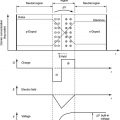

Full access? Get Clinical Tree


