Fig. 2.1
Renal cyst. Sagittal sonographic image of the left kidney demonstrates a well-circumscribed, anechoic, thinly walled lesion with posterior acoustic enhancement (black arrows), a finding which is often used to definitively characterize a lesion as cystic. At the lateral edges of the enhanced echoes, there is a faint shadow representing edge (refraction artifact) which results from bending of the sound wave from its expected path
Attenuation
Attenuation refers to decreases in sound beam strength as it travels through tissue. Frequency is a determining factor of attenuation, and the higher the frequency of the sound wave, the greater the attenuation. The penetrating power of sound is therefore limited at higher frequencies. Tissue density is another determining factor of attenuation. Reflections and refractions are some of the reasons for this phenomenon. Another is the conversion of the sound energy to heat.
Acoustic shadowing is an example of attenuation differences in action. The term refers to lost through transmission of the sound beam. An example is seen in renal calculi which both absorb and reflect the sound beam, resulting in acoustic shadows posterior to the calculus, due to marked attenuation of the sound beam (Fig. 2.2). In contrast, posterior acoustic enhancement is a phenomenon produced when attenuation of a structure is less than that of surrounding tissue, resulting in greater amplitude of the beam posterior to the structure. This is falsely displayed as an increase in echogenicity of the tissue posterior to the weakly attenuating structure. In clinical practice, this is commonly seen in the setting of a simple renal cyst (Fig. 2.1) or any other fluid-containing structure, such as the urinary bladder [2–5]:
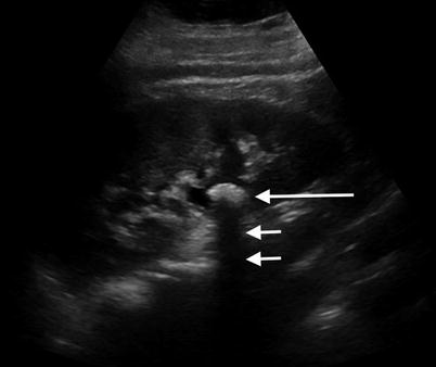
Fig. 2.2
Renal calculus. Sagittal sonographic image of the right kidney demonstrates a calcified renal stone (large white arrow) with the classic appearance of an echogenic lesion causing posterior acoustic shadowing (small white arrows)
Attenuation coefficients for selected tissues at 1 MHz
Material attenuation coefficient (dB/cm)
Water 0.0002
Soft tissue 0.3–0.8
Fat 0.5–1.8
Bone 13–26
Air 40 [4]
Pulse-Echo Imaging Modes
Amplitude Mode (A-Mode)
Motion Mode (M-Mode)
Echo signal amplitudes are modulated according to levels of brightness and are displayed in a variety of shades of gray. The ultrasound beam is fixed at one position yet is observed in real time while scanning, allowing for the imaging of the motion of moving structures. A clinical example of M-mode use is in echocardiography, in which real-time evaluation of myocardial motion is performed [2, 3, 5].
Brightness Mode (B-Mode)
This mode produces a 2D image via modulating the echo signal amplitudes to various levels of brightness. This allows echoes to be displayed as lines with the imaged composed of “point-by-point variations in brightness level aka various shades of gray.” In practice, structures that are more sound wave reflective appear more hyperechoic than those that are less reflective. Furthermore, the pulse line can be swept across tissue planes and produce cross-sectional imaging in the 2D plane [2, 3, 5].
Transducers
The sound beam is created by the transducer which makes use of a phenomenon called the piezoelectric effect to convert electrical energy into vibrational energy. This is accomplished by alternating electric current to the transducers crystal which causes expansion and contraction. Thus this produces vibrations and therefore sound waves. In addition to producing the sound beam, the transducer is also capable of receiving the reflected sound waves, referred to as echoes. Upon receipt, the crystal vibrates at the received echoes’ frequency and converts that frequency into electrical current which is processed and converted into the ultrasound image [2, 3, 5].
Array technology allows for electronic focusing to a variety of depths with multiple focal zones from the same transducer. These capabilities yield better image quality/resolution/sharpness. Older transducers, in contrast, generated the sound beam with one element, causing the beam to converge at a focal zone, proximal to which was termed the near field and distal to which was termed the far field, where the sound waves diverged. The depth of the focal zone was determined by the characteristics of this single element [2, 3, 5].
Linear Array
Linear array transducers are composed of parallel scan lines which are perpendicular to the surface of the transducer. These utilize higher frequencies and provide high-resolution imaging of fascial planes that lay parallel to the skin surface. Linear arrays are most commonly used for imaging superficial and small parts and for musculoskeletal and vascular imaging where there is a need for highly detailed images [3, 5].
Curvilinear Array
These transducers are composed of crystals aligned in a convex arrangement, and thus, the scan lines diverge as the sound beam travels deeper into the scanned tissue. They typically utilize lower frequencies, allowing for deeper tissue penetration compared to linear high-frequency imaging. Interpolation is often required to fill in the gaps in the image produced by the diverging sound waves. The advantage of the curved array is that it produces a larger field of view for deeper tissue structures. It is often used for abdominal and obstetric imaging [3, 5].
Phased Array
These specialized transducers are composed of many more, often approximately 100, elements. They produce pulsed beams for each scan line, and thus, the beam can be steered in a different fashion than, for example, the linear array. The transducer also has a rather narrow face and the end result of its image formation is one with a large lateral view of deeper tissue [3, 5].
A variety of modified transducer arrays are available for specialized imaging tasks by taking advantage of different focus strategies for specific anatomic regions. For example, endorectal probes are utilized for transrectal prostate biopsy, and endoesophageal probes are utilized for transesophageal echocardiography.
Image Resolution
Lateral Resolution
Lateral resolution refers to the minimum measurable separation of objects that lay parallel to the face of the transducer. Objects appear separated if their separation is in fact greater than the width of the sound beam. Higher-frequency transducers produce a longer near field, which is the narrowest portion of the beam. The near field is the region at which lateral resolution is the greatest. Higher-frequency transducers produce a narrow beam width, which decreases the amount of beam dispersion, which occurs in the far field. This thus allows for better lateral resolution [3, 5]. Focusing the beam further enhances lateral resolution by narrowing the beam width at a selected area of tissue.
Axial Resolution
Axial resolution refers to the minimum measurable separation of objects along the axis of the beam. The beam pulse length is the principal factor. A pulse length longer than twice the object separation will not generate resolvable echoes. Two basic techniques in which short pulses are generated are through broad bandwidth pulses and high-frequency beams. Therefore, broad bandwidth and high-frequency transducers are capable of producing short pulses and thus higher-resolution imaging [3, 5].
Elevational Resolution
Elevational resolution refers to slice thickness and is the same entity as lateral resolution but refers to the plane orthogonal to the image plane. The major contributing factor is beam width in this plane. Electronic control of transducers allows for other features that optimize image resolution. In modern ultrasound machines, the majority of these are automated upon selection of specific imaging protocols. These have the potential to improve image quality through the focus and filter of an echo upon its return to the transducer and help to enhance lateral resolution of the image by decreasing noise from the outer edges of the beam. Examples include:
Receive focus: received echoes from single pulse are electronically focused to account for location in the beam.
Dynamic aperture: aperture or sensitive area of the transducer is modified on reception to help eliminate side lobe or scattered signals from the edge of the beam.
Transmit Power Control
The modulation of transmit power affects the pulse amplitude from the transducer. Stronger, greater amplitude pulses produce stronger returned echoes. This improves signal to noise ratio and increases the maximum depth of imaging. There is a potential risk of adverse bioeffects with prolonged exposure to high transmit power pulses in diagnostic ultrasonography; however, there are no reported confirmed cases. Nevertheless, “prudent and conservative” use of diagnostic sonography under the ALARA principle encourages the use of the lowest possible transmit power to produce diagnostic quality images [1, 5].
Frequency Selection
The ultrasound transducer has a broad frequency bandwidth which corresponds to the emitted pulse. The “nominal” frequency of a transducer is usually the center frequency of the bandwidth. As the frequency is increased, spatial resolution improves; however, the penetration of the beam decreases. Conversely, lower frequencies allow for greater penetration albeit with poorer spatial resolution. Thus the selection of transducer frequency is dependent on the clinical situation and requires a balance between the desired depth of penetration and spatial resolution [1, 5].
Doppler
Doppler ultrasound allows for clinical assessment of the presence or absence of flow within a vessel or tissue and can give information on blood flow direction, pulsatility, and velocity. Doppler ultrasound processes frequencies of returning echoes from the imaged tissue to compose an image, as opposed to gray-scale sonography that utilizes the amplitude of the returning echoes. The foundation of Doppler ultrasound is the so-called Doppler effect. This refers to the change in frequency of a sound wave that occurs due to the relative motion of either the source, the observer (transducer), or the tissue medium. A commonly used example is the way in which the sound pitch of a moving train’s whistle changes as it passes an observer. Clinically, blood cells act as moving reflectors of the ultrasound beam, and thus, blood flowing toward the transducer reflects the beam at a relatively higher frequency than blood flowing away [1, 6, 7]. The same transducers utilized for gray-scale imaging are capable of Doppler imaging. Three major Doppler imaging techniques are utilized clinically and discussed in the following sections.
Pulsed Wave (Spectral) Doppler
This is based on the velocity of a selected sample volume of blood flow and generates a waveform based upon directionality of flow: Flow toward the transducer is plotted above the baseline, and flow away from the transducer is plotted below. The velocity of the blood flow is demonstrated as the wave amplitude, and the characteristics of the waveform shape allow clinical inferences to be made about the type of flow. Spectral Doppler allows for the analysis of multiple different vessels at different depths and provides a high range of resolution and specificity due to the sampling component [1, 5, 7].
Color Doppler
This is a 2D depiction of blood flow which is superimposed on a gray-scale image of the tissue imaged. Relative direction of flow is depicted and based upon the average velocity of the blood. By convention, red typically is used for blood flowing toward the transducer and blue used for blood flowing away, although these settings can be easily switched. Color Doppler allows for the characterization of the quality of the blood flow, for example, turbulent vs. laminar flow. The intensity of the color display also varies as a depiction of the flow intensity (i.e., lighter shades depicting higher-frequency shifts). Objects that are stationary are depicted in gray scale only. Color Doppler therefore yields important clinical information about the overall flow to the imaged region and can help one choose where to place a spectral Doppler sampling window. The advantage of color Doppler is that it is a relatively easy technique for confirming the presence or absence of flow and visualizing small vessels, such as in the testes. Limitations include lower spatial resolution vs. gray-scale imaging as well as its relative insensitivity to slow flow or flow in small-caliber vessels for which spectral Doppler is superior [1, 5, 7].
Power Doppler
Power Doppler provides a display of the strength of the Doppler signal in contrast to the average shift of frequency. The color and shade displayed on the image are dependent upon the volume of the flowing blood. The primary advantage of power Doppler is a high sensitivity for detecting flowing blood. It is especially useful for the detection of slow flow or blood within very small vessels. Power Doppler is not susceptible to aliasing, in contrast to spectral and color Doppler. Unlike color and spectral Doppler, there is no reliance upon the Doppler angle, and thus, images of vessels in the perpendicular plane are possible to obtain. The disadvantages are that power Doppler does not provide any information about the directionality or velocity of blood flow. Power Doppler is vulnerable to motion, either of the transducer or of the tissue which manifests as an intense flash of color on the monitor, termed flash artifact [1, 5, 7].
Ultrasound Applications for the Genitourinary System
Normal Renal Anatomy
The normal ultrasound appearance of the kidneys is one of paired retroperitoneal structures. Each kidney is enclosed by a dense capsule, which itself is then surrounded by perinephric fat enclosed in Gerota’s fascia. Sonographically, the kidney is conventionally imaged in the transverse and sagittal planes. Normal renal parenchyma in the longitudinal image is homogeneous with the normal cortex appearing more hyperechoic relative to the medulla. The medullary pyramids are thus hypoechoic in appearance relative to the cortex. They abut the renal sinus fat, which appears relatively hyperechoic. The center of the longitudinally displayed kidney is a complex of rather dense-appearing structures which include the peripelvic fat, renal vessels, lymphatic vessels, and normal collecting system. The normal vascular pedicle and the small intrarenal vasculature and renal perfusion are often well visualized and interrogated with the use of Doppler imaging to demonstrate the quality and quantity of flow [2, 8].
Renal Masses
Simple cysts (Fig. 2.1) are the most common benign adult renal mass, and ultrasound has proven an effective tool in evaluating renal cysts, allowing for differentiation from other cystic and solid renal masses. Simple cysts are commonly round, demonstrate a clearly defined thin wall, and lack internal echoes. The latter of these produce a characteristic feature known as posterior acoustic enhancement. The presence of internal septations, nodular components, internal echoes, and calcifications are more worrisome features. Complex or septated cystic renal masses as well as solid masses raise suspicion of neoplasm (vs. abscess or hematoma) [2, 9, 10].
Sonographic characteristics of solid lesions include delineation of the posterior wall, lack of through transmission, and internal echoes. In the past, color flow and Doppler imaging were utilized to help differentiate different types of solid renal neoplasms. Ultrasound characterization of solid renal masses is more limited compared to cystic lesions, and more advanced imaging modalities such as CT and MR are indicated for further evaluation [2].
Angiomyolipoma (Fig. 2.3) is a benign, fat-containing renal mass that has a characteristic sonographic appearance. Lipid-rich lesions will demonstrate a characteristic homogeneous hyperechoic appearance and allow for a presumptive diagnosis, although infrequently this appearance can overlap with renal cell carcinoma. Therefore, additional imaging with CT is necessary to confirm the presence of macroscopic fat [9, 10].
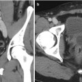
Fig. 2.3
Renal angiomyolipoma. Sagittal gray-scale sonographic image of the right kidney (a) demonstrates a rounded, hyperechoic, and nonshadowing solid mass at the upper pole of the kidney (arrow), consistent with angiomyolipoma. Accompanying non-contrast axial T1 in-phase (b) and T1 fat-saturated images (c) demonstrate the same mass to have high signal on the T1-weighted image (b) and diffuse signal loss (c) on the fat-suppressed image, confirming the diagnosis
Ultrasound can offer useful evaluation of mass lesions of the renal collecting system. Commonly, calcified calculi (Fig. 2.2) demonstrate the classic appearance of an echogenic focus with posterior acoustic shadowing. Even poorly or noncalcified calculi tend to demonstrate a hyperechoic echotexture and often shadow. Other lesions such as hematoma and neoplasm are often distinguishable from calculi, but their definitive diagnosis is better obtained via urologic procedures or additional imaging [2].
Overall, sonography is limited in its ability to stage the extent of malignant disease, which is better accomplished with CT and/or MRI.
Renal Failure
Ultrasound is commonly employed in the evaluation of renal failure as obstructive uropathy is an easily identifiable cause. Hydronephrosis (Fig. 2.4) is the hallmark of renal failure due to obstruction and is characterized by the loss of the normally echogenic renal sinus which is replaced by a dilated hypoechoic collecting system. The level of dilatation of the calyces, infundibula, renal pelvis, and proximal ureter as well as the degree of parenchymal thinning can aid in inferring the degree and chronicity of the obstruction. Differential diagnostic considerations include parapelvic cysts, megacalyces, calyceal diverticula, and extrarenal pelvises. Post-intervention, ultrasound serves as an inexpensive and rapidly performed imaging study to assess for residual collecting system dilatation [2, 8].
Fig. 2.4
Hydronephrosis. Sagittal (a) and transverse (b) sonographic images of the right kidney. The renal collecting system is symmetrically dilated, including dilatation of the renal calyces and central collecting system
Renal Transplant
The pelvic and superficial location of the transplanted kidney allows for it to be interrogated well by sonography. Postoperative perinephric collections, such as lymphoceles, urinomas, and hematomas, are usually identifiable. With decreased urine output, changes in renal volume and perfusion can be evaluated with sonography and allow for distinguishing obstruction from other transplant-related pathologies [2, 11].
Assessment of renal function is best accomplished with radionuclide imaging as the gray-scale ultrasound appearance in renal failure is rather nonspecific. Such findings include renal enlargement, increased cortical thickness, increased/decreased cortical echogenicity and loss of corticomedullary differentiation, prominent pyramids, thickness of the collecting system, and central sinus effacement. Ultrasound does however serve as an important tool in evaluating vascular complications of transplantation. Although conventional angiography remains the gold standard for the diagnosis of vascular complications, spectral and color Doppler ultrasound provide an excellent and noninvasive assessment of affected vessels. Pathologies typically encountered include renal arterial or venous occlusion or stenosis and pseudoaneurysms and arteriovenous fistulae [11].
Renal artery stenosis (Fig. 2.5) is the most common vascular complication of transplantation, reported in up to 10 % of patients. Color Doppler interrogation of a stenotic segment will demonstrate areas of focal aliasing. These regions can then be selected for spectral Doppler evaluation to quantify the degree of stenosis, which can then be evaluated with duplex Doppler techniques to characterize and grade the abnormality. Spectral Doppler criteria for significant stenoses include (a) velocities greater than 2 m/s or focal frequency shift greater than 7.5 kHz (when a 3-MHz transducer is used), (b) a velocity gradient between stenotic and pre-stenotic segments of more than 2:1, and (c) marked distal turbulence (spectral broadening). The presence of the classically described “tardus parvus” (“late, small” in Latin) waveforms may further support the diagnosis; however, they are not always present. If there is no significant flow abnormality demonstrated, renal arterial stenosis can be excluded [10–12].
Fig. 2.5
Renal artery stenosis. Spectral Doppler sonographic images of the right renal artery, (a) at the level of a high-grade stenosis in the distal renal artery and (b) at the level of the segmental arteries, distal to the stenosis. (a, b) Abnormally high velocity is demonstrated at the level of the renal artery stenosis, while the arterial waveforms distal to the stenosis (b) show an abnormally delayed systolic upstroke with low amplitude (“tardus parvus”) with corresponding low velocity. (c) Digitally subtracted image from renal arteriogram in the same patient shows a high grade mid-arterial stenosis (arrow). Normal renal arterial waveform. (d) A normal low-resistance waveform and velocity are demonstrated in the left renal artery in a different patient. Note the rapid systolic upstroke, with peak <150 cm/s and continuous low-resistance flow throughout diastole
Urinary Bladder
The normal sonographic appearance of the urinary bladder is a globular, hypoechoic structure whose shape is variable, depending on the level of distension and the patient’s position at the time of examination. The wall appears hyperechoic, smooth, and diffusely symmetric in thickness. When the normal bladder is distended, the lumen should be anechoic [2].
Bladder tumors can sometimes be visualized sonographically. Polypoid lesions (Fig. 2.6) appear as intraluminal soft tissue projections which are fixed to the bladder wall and are nonmobile with patient change in position, in contrast to mass-like lesions such as hematoma and calculi. Tumors are solid lesions in contrast to ureteroceles which, although they are also fixed to the bladder wall, have a distinct sonographic appearance with a thin echogenic wall and anechoic (cyst-like) center. Calculi within the bladder behave sonographically as in other areas of the GU tract with hyperechoic echotexture and posterior acoustic shadowing. Calculi will move as the patient changes position unless lodged at the ureterovesical junction [2].
Fig. 2.6
Urinary bladder neoplasm. Transverse gray-scale (a) and color Doppler (b) sonographic images of the urinary bladder demonstrate a solid, exophytic mass within the urinary bladder lumen (arrow (a)) without any posterior acoustic shadowing and (b) with internal vascular color Doppler signal, indicative of a solid, vascularized lesion, rather than blood clot, adherent debris, or non-shadowing calculus
Prostate
The normal sonographic appearance of the prostate is a symmetric triangular ellipsoid gland circumscribed by a fibrous capsule. The capsule itself appears as a continuous thin and hyperechoic layer of tissue. Internally the prostate demonstrates multiple fine diffuse homogeneous echoes which likely result from the interfaces of the myriad of small glands within. The posterior peripheral zone systolic velocity can typically be differentiated from the more anterior peripheral zone, the central and transition zones, and the fibromuscular stroma [2].
Transrectal ultrasound has been shown to be useful in evaluating benign and malignant prostatic disease and plays a valuable role in biopsy and assessment of treatment of patients with prostate carcinoma (Fig. 2.7c). Note, however, that transrectal ultrasound is useful only to localize the prostate and not for the identification of lesions [2, 12–15].
Fig. 2.7
Prostate carcinoma. (a) Axial T2- and (b) diffusion-weighted images of a right central prostate gland carcinoma (arrows (a, b)). (c) Transverse transrectal sonographic image of the prostate obtained during transrectal fusion biopsy demonstrates the lesion as a heterogeneous hypoechoic mass (arrow)
Commonly used transrectal transducers used for prostate imaging range in frequency from 6.0 to 7.5 MHz. The higher frequency allows for detailed images; however, penetration of the beam is limited and thus the anterior prostate is often incompletely visualized. Most transducers are biplanar and provide images in the transverse and sagittal planes. The transverse plane allows for better visualization of the lateral margins, while the sagittal plane provides better images of the gland’s apex and base [2, 12, 14, 15].
Currently, sonographic diagnostic evaluation of the prostate has a limited role in comparison with MRI (Fig. 2.7a, b). The anterior prostate is often insufficiently visualized, and thus lesions in this region can go undetected. Additionally, many benign lesions as well as normal structures have similar sonographic appearances to small malignant lesions. Some carcinomas, in fact, are completely isoechoic and therefore the utility for diagnostic prostatic ultrasound is quite limited. It is becoming increasingly evident that supplementing the work-up of prostate cancer with prostate MRI when used in conjunction with transrectal ultrasound-guided biopsy will result in much higher yield for tissue diagnosis of malignancy [2, 12–15].
Penis
Sonographic evaluation of the penis is ideally conducted with a high-frequency linear transducer. This provides good visualization of the two corpora cavernosa, which are demonstrated as symmetric structures of homogenous mixed echogenicity which is due to the many interfaces of the vascular sinusoids. In contrast to the two corpus cavernosa, the corpus spongiosum normally appears mildly hypoechoic in comparison. The fibrous tunica albuginea appears as a hyperechoic line forming the intercavernous septum and provides a region of posterior acoustic shadowing between the corpora. Color and spectral Doppler sonography can evaluate penile vessel patency and characterize blood flow [2, 16].
Most applications of penile sonography occur in the acute setting. Acute conditions of the penis lend themselves to evaluation with ultrasound due to its wide availability and the real-time assessment it provides. Penile fracture results from tearing of the tunica albuginea leading to rupture of the corpora. Ultrasound is capable of demonstrating tears and the extent of the associated injury. The tear is visualized as a segmental discontinuity of the tunica albuginea, and associated hematoma may be visualized deep to the Buck fascia or subcutaneously. A secondary sign suggesting associated urethral injury is the presence of echogenic air in the cavernosa. The evaluation of the urethra with ultrasound is however limited, and when there is clinical concern of urethral injury, retrograde urethrography is indicated [2, 16].
Scrotal Ultrasound
The scrotum and its contents are superficial structures and thus well visualized with sonography. Scrotal pain and swelling prompt evaluation and sonography allows for differentiation between tumors, orchitis/epididymitis, torsion of the spermatic cord, and traumatic lesions such as fracture. Testicular and paratesticular malignant tumors are typically hypoechoic in appearance, and identification of such a mass demands surgical intervention in most scenarios. Nonseminomatous tumors can demonstrate increased vascular flow on Doppler imaging, while seminomas characteristically demonstrate homogeneous echotexture in contrast to embryonal tumors. Epididymitis is typically characterized by an enlarged and hypoechoic epididymis due to edema with hypervascularity on color Doppler imaging. Often, there is a reactive hydrocele accompanying the lesion. Epididymo-orchitis can have similar findings, as well as an enlarged and hypervascular testis [2, 17].
Clinically, distinguishing between testicular torsion (Fig. 2.8) and epididymo-orchitis can be difficult, and ultrasound has been found to be quite useful. In early torsion (approximately 1–3 h), echogenicity of the testes appears normal. As time goes on, there is enlargement of the torsed testis, and it will appear increasingly heterogeneous in echotexture. Evaluating the spermatic cord in suspected torsion is critical as a torsed cord can be visualized in the external inguinal orifice and aid in making the diagnosis. The intrascrotal portion of the torsed and edematous cord can appear as a rounded echogenic extratesticular mass. The orientation of the cord, testis, and epididymis can be inverted. The diagnosis is further strengthened with the evaluation of testicular blood flow, with the affected side demonstrating abnormal or absent flow compared to the normal testis. Comparative imaging with transverse views, including pulsed Doppler imaging can yield important information regarding decreased or reversed diastolic blood flow to the affected testis when compared to the normal side [17].
Fig. 2.8
Testicular torsion. Gray-scale and color Doppler images of the testes and gray-scale image of the spermatic cord in a young man presenting with acute right scrotal pain. (a) Color Doppler side-by-side transverse image demonstrates the absence of vascular flow to the right testicle compared the normal left testicle as manifested by the lack of color signal. (b) Transverse image demonstrating twisting of the spermatic cord (arrow)
Traumatic injury to the scrotum lends itself to sonographic evaluation as the pain and swelling often limit physical examination. Findings include extratesticular hematoma and testicular rupture, the latter of which should be suspected in the case of poorly defined testicular margins and/or disruption of capsular blood flow. The echotexture of extratesticular/scrotal hematoma evolves over time with a more echogenic acute appearance transitioning to a more hypoechoic appearance in the subacute and later stages [17].
Varicocele
A varicocele (Fig. 2.9) will appear as a series of tortuous anechoic tubular structures either around, above, or below the testis. There is some variation in the caliber of the vessels used by different authors, ranging typically from 2 to 3 mm. When utilizing color Doppler sonography at rest, blood flow within a suspected varicocele may be too slow for detection. With utilization of the Valsalva maneuver, the varicocele will enlarge and demonstrate reversal of flow. Color Doppler sonography is the accepted gold-standard technique for varicocele assessment as it provides accurate diagnosis and can also be used to stage lesions [18].
Fig. 2.9
Varicocele. Gray-scale (a) and color Doppler (b) sonographic images of the left testicle and an adjacent hydrocele. An extratesticular plexus of tortuous vessels (arrows (a, b)) is demonstrated with dilatation of the individual vessels upon Valsalva maneuver. Incidentally noted testicular microlithiasis can also be seen, manifested by scattered echogenic intratesticular foci
Computed Tomography (CT): Physical Principles and Genitourinary Applications
Physical Principles
The first CT scanner was developed by Sir Godfrey Hounsfield in Middlesex, Great Britain. In 1973, the first CT scanners were used clinically. Houndsfield and Allan Cormak were awarded the Nobel Prize in Medicine in 1979 for the development of CT technology [1, 19]. In the following decades, with constant advances in technology and computational power, cross-sectional imaging has revolutionized the practice of medicine, due to its capability to evaluate disease processes throughout the body in a noninvasive manner.
There are many urologic applications of CT, including, but not limited to, detection and characterization of renal stone disease; obstructive uropathy; benign and malignant tumors of the adrenals, kidneys, and upper and lower urinary tracts; traumatic injury; infection and its complications; and assessment of renal artery disease. Technologic advances over the years have greatly increased the capabilities of CT and have resulted in markedly greater speed of acquisition, anatomic coverage, and the ability to obtain dynamic contrast-enhanced images, all of which have worked to increase its diagnostic accuracy and image quality. This has also led to the development of newer applications, such as dual-energy CT, CT angiography, and CT urography. A drawback to the use of CT is its use of ionizing radiation, which results in a relatively large radiation dose. In recent years, however, dose reduction techniques have been implemented on a wide-scale basis, which have the potential to significantly reduce the dose from routine CT imaging.
A fundamental limiting factor of plain film radiography is that a three-dimensional object is reduced to a two-dimensional image, with the potential for multiple structures of varying radiodensity to be superimposed on one another, with the potential for the anatomy of interest to be obscured. Two distinct and extremely important advantages of CT over plain film radiography are (1) acquisition of a cross-sectional image with removal of any superimposed structures and (2) almost complete elimination of radiation scatter, which results in much greater sensitivity to differences in x-ray attenuation, thereby allowing excellent contrast between soft tissue structures. A CT examination is made up of multiple images, each one containing visual information from narrow anatomic sections through the imaged section of the body. The penetrating x-ray beam is collimated (shaped) into a very precise width [1, 19].
CT scanners are made up of two major components: the scanning component and computer components. The gantry consists of the scanning components, which surround the central aperture through which the patient is scanned. The computer components are located in the CT scanner control room. The scanning component includes the generator or power source, x-ray tube, collimators, detectors, data acquisition system computer components, image reconstruction, and scanner console.
Each detector, along with the focal spot of the x-ray tube, defines a ray. The detector measures the intensity of the x-rays within its ray. The intensity of the beam within each ray depends on the amount that x-rays are attenuated in the tissue through which it passes. Attenuation is a measurement of the fraction of radiation removed in passing through tissue. The attenuation of each boxlike element, or voxel, in the plane being scanned is measured by using many different rays acquired from many different angles over the course of the scan. The linear attenuation coefficient of a material indicates how strongly it absorbs or scatters (attenuates) x-ray photons. The linear attenuation coefficient depends on three properties: atomic number, physical density, and photon energy. The creation of a CT image is reliant upon the different attenuation characteristics of various tissues in the body [1, 19].
Once image detectors have assembled the data from each ray, images are reconstructed via analytical and iterative methods. The most commonly used reconstruction method is filtered backprojection, which has been used in the earliest CT scanners and is still used today. Filtered backprojection essentially determines the average density of each pixel by collecting sets of rays called projections, which are made across the patient in a particular direction in a section plane. Multiple projections are needed to determine average attenuation at each point, using rotational intervals of less than 1° [1, 19].
CT images are composed of gray-scale values, with each element of the image (pixel) assigned a gray-scale value dependent upon its average attenuation. Denser materials will cause greater attenuation of photons and will be brighter (whiter) on the CT image, while images that are less dense will be darker (blacker). Density measurements are standardized using the Hounsfield scale, in which water has a Hounsfield unit of zero, with other tissues ranging from −1000 (air) to +2000 (bone). Any voxel that has attenuation greater than water will have a positive HU value, and voxels which have attenuation less than water will have a negative HU. An attenuation value of specific tissue can be easily obtained by placing a cursor over the region of interest (ROI) at the workstation, for which the computer can average the attenuation of the voxels within the cursor. Attenuation values play great importance in tissue characterization and diagnosis and must be precisely calibrated on a regular basis [1, 19].
Detector arrays in multislice scanners are two dimensional. The number of detectors in the z-direction (in the head-to-toe direction of the patient) determines the maximum number of slices which can be simultaneously acquired. In a single-slice scanner, the slice width is determined by the width of the collimator. In multislice scanners, the slice width is determined by the width of the individual detectors. For instance, in a system with 64 detectors which are 0.625 mm in width, the slice thickness is 0.625 mm [19]. In actual practice, thicker slices are usually reconstructed for routine interpretation; however, thin sections are stored at the CT workstation and are available for review, if necessary.
Many imaging acquisition parameters determine image quality and patient dose. Two important acquisition parameters that affect radiation dose and image quality are peak tube voltage (kVp) and effective mAs. The effective mAs is the tube current (milliamperes) multiplied by the length of time that a given point in the patient is in the beam (seconds). The energy of the most energetic x-ray photon in the beam is always equal to the kVp. Pitch is another important acquisition parameter: this refers to the table movement per tube revolution divided by the beam width. Adjustments in pitch affect scan time, z-axis resolution, and radiation dose [1, 19].
Prior to the introduction of helical CT technology, scanners operated in axial or incremental mode. In axial CT scanners, the CT table is stationary during image acquisition, with the tube and detectors making one complete rotation. The x-ray beam is then turned off and the table repositioned [1, 19].
The design of modern CT scanner has been modified so that there are no hardwired connections between the generator and x-ray source and between the detector array and computer. This is achieved by slip-ring technology. Slip-ring technology, as well as advances in x-ray tube design and computer speed, made the development of helical scanning possible. Helical CT allows for uninterrupted motion of the x-ray source and the detector array, which rotate in a complete 360° arc around the patient. Simultaneously, the CT table (and patient) is moving in a continuous manner and at a predetermined speed [1, 19]. The result of these two different movements is that the beam takes a helical path through the patient. Helical scanners are capable of much faster scanning times and thinner slice acquisition than incremental CT scanners [19]. This improved temporal resolution has enabled dynamic studies after the administration of a bolus of intravenous iodinated contrast, whereby the entire abdomen and pelvis can be scanned on the order of seconds and images can be obtained in various phases of interest for a particular indication. For example, a typical examination for the evaluation of a renal mass would include arterial, nephrographic phases and sometimes excretory (pyelographic) phases as well as an unenhanced acquisition.
Dual-Energy CT
Dual-energy CT (DECT) scanners are built with two x-ray source/detector arrays. The tube voltage (kVp) settings for the two sources differ, resulting in two separate attenuation maps for the same object, one at a high energy level and one at a low energy level. As mentioned above, the linear attenuation coefficient of a specific material is dependent upon three properties: atomic number, density, and photon energy. DECT uses information obtained from both the high and low energy arrays to assess the rate of change in the linear attenuation coefficient of the structure being analyzed. As various elements and compounds commonly found in the human body have unique linear attenuation curves over a spectrum of energy, DECT is capable of providing information regarding specific chemical composition [20].
There are several ways in which the data obtained from DECT can be exploited to provide useful clinical and diagnostic information. Material-specific images can be formed by targeting a specific material’s linear attenuation curves and removing it from the image. Common base materials targeted by DECT include water, iodine, and calcium. As enhancement on CT is produced from the effects of iodinated contrast medium, subtracting iodine results in a “virtual” non-contrast image, so that a single dual-energy scan could potentially replace two single-energy scans (pre- and post-contrast) [20]. This could have application in the evaluation of renal masses, calculous disease, adrenal nodules, and any other scenario where non-contrast images are necessary for lesion characterization or visualization. An additional benefit of virtual non-contrast images would be radiation dose reduction, due to elimination of a separate unenhanced acquisition.
Conversely, iodine-specific data sets (iodine maps) can be obtained. These are composed exclusively of the contribution of iodine to the image and may also be efficacious in renal mass characterization and other scenarios [21]. By enabling better visualization of iodine signal, enhancement within a mass may be more easily diagnosed on iodine-specific images. Studies have so far shown promising results for the use of virtual non-contrast and iodine-specific images in differentiating cystic from solid renal masses [21–23]; however, these techniques will require further study and validation. Future advances and refinements in dual-energy technology may even surpass the diagnostic capabilities of conventional, single-source CT.
Virtual non-contrast images have also shown promise in characterizing adrenal nodules [24, 25]. This is a promising development given the high frequency of adrenal nodules found on contrast-enhanced CT scans, which often need repeat CT examination with unenhanced images to better characterize.
Another active area of investigation of DECT is in renal stone characterization. DECT makes use of the distinctive absorption patterns of various stone components at both high and low energy levels to identify specific chemical composition [20]. This can expedite the work-up of renal stone disease, which can often involve lengthy laboratory and imaging investigation. Knowledge of stone composition can help improve treatment, as management of different stone types differs. DECT has shown to be reliable in differentiating uric acid stones from non-uric acid stones [20] and shows promise in the differentiation of other calculi (cystine, struvite, calcium oxalate monohydrate/calcium oxalate dihydrate/brushite, and hydroxyapatite/carbonate apatite calculi) [26, 27].
Applications of CT in the Urinary Tract
Kidneys
There are numerous indications for the use of CT in the evaluation of renal pathology. Some of the more common reasons include renal mass characterization, renal cancer staging, stone disease, trauma, inflammatory/infectious processes, obstructive uropathy, vascular disease, congenital urinary tract anomalies, and postoperative evaluation.
CT is a highly accurate modality for renal mass evaluation. Since the differential diagnosis often revolves around differentiating between a cystic and solid mass, the key element of such evaluation is the presence or absence of contrast enhancement [28]. Benign renal cysts are typically uniformly low in density (at or near the attenuation of water) on CT, with an imperceptible wall and no septations or mural nodules; however a significant minority will appear as high-attenuation lesions on CT due to the presence of hemorrhagic or proteinaceous debris. Because the density of these lesions (greater than 20 HU) overlaps with solid nodules, they cannot be differentiated by unenhanced or contrast-enhanced CT alone. Rather, both unenhanced and enhanced images must be acquired in the same sitting, with HU measurements obtained from both series. At this time, there is no true consensus on what constitutes significant enhancement; however, a threshold of >20 HU is used by some experts, with a 10–20 HU difference considered to be equivocal [28]. In the case of an enhancing soft tissue mass with no visible fat, there are no reliable CT findings to help differentiate a benign soft tissue mass, such as an oncocytoma or lipid-poor angiomyolipoma, from a renal cell carcinoma (RCC). Lymphoma and metastatic disease can also have a similar appearance to RCC, and attention to medical history and extrarenal findings must be made in order to make an accurate diagnosis. Nonneoplastic mimics of renal cell carcinoma include focal pyelonephritis, “pseudotumor” arising from congenital lobulation of the renal contour or from normal parenchyma adjacent to scarred cortex, and IgG-4 disease [29].
Artifacts, such as beam hardening from a patient who is unable to position his/her arms away from their sides or from pseudoenhancement, can give spurious results. Pseudoenhancement is a well-known artifact on CT, which causes increase in attenuation measurements in renal lesions on intravenous contrast-enhanced CT. This is due to an incorrect image reconstruction algorithm in areas adjacent to high-attenuation structures (in this case, the avidly enhancing renal parenchyma), with small, intraparenchymal lesions most likely to be affected [30, 31].
Cystic renal lesions are ubiquitous in the adult population, with simple cysts comprising the overwhelming majority of these masses. Cystic neoplasms do, however, arise in the kidney; therefore, the density (HU) measurement and internal composition of all cystic renal masses must be carefully assessed. The presence of enhancing septations and nodules increases the likelihood of a cystic neoplasm. The Bosniak classification of cystic renal masses categorizes lesions based on their morphology. Bosniak criteria include density, number, and thickness of septations; wall thickness; and soft tissue nodules (Fig. 2.10). The presence or absence of enhancement must be carefully assessed, as benign hemorrhagic cysts can have many of the features of a cystic neoplasm; however, any internal components should not enhance [28].
Fig. 2.10
Cystic renal cell carcinoma. Axial unenhanced (a, b) contrast-enhanced CT images demonstrates a large cystic left renal mass with nodular enhancing components (black arrows). Enhancement within a renal mass must be confirmed by comparison with unenhanced CT images. Also note two small fat density right renal lesions representing angiomyolipomas (white arrows)
Angiomyolipomas are well assessed on CT and can be diagnosed when a renal mass contains macroscopic fat. This is a key element of renal mass characterization, as it is extremely rare for a renal cell carcinoma to contain fat. An unenhanced thin-section CT is the most sensitive test for fat detection and should be performed if fat is suspected in an enhancing renal mass. A small minority of angiomyolipomas will either contain no fat or an insufficient amount of fat to be detected at CT. Although these lesions often have features on CT that may suggest the diagnosis, they cannot be reliably distinguished from renal cell carcinoma without biopsy or surgery [28].
In cases of known renal malignancy, CT is an accurate modality for staging. The renal vein and IVC can be assessed for the presence and extent of tumor invasion. Tumor thrombus can often be distinguished from bland thrombus by enhancement in the former; however, there are limitations of both CT and MRI in assessing for invasion of the IVC wall, which can significantly impact prognosis [32


Related posts:
Stay updated, free articles. Join our Telegram channel
Full access? Get Clinical Tree
